SA-CVA: turning a regulation into code
The capital formula for CVA risk is forty lines of arithmetic once you have the sensitivity vector. Getting that vector is the hard part: seven risk factors, each one the derivative of a full counterparty-exposure simulation. Real numbers from a run: one adjoint sweep vs 28 re-simulations, 113x apart, agreeing to 0.002%.
How much capital does a bank need against the risk that a counterparty's credit-valuation adjustment moves against it? The regulatory formula for that number is short. Getting the seven numbers it needs is not — each one is the derivative of an entire Monte-Carlo exposure simulation, not a cheap repricing.
The whole story
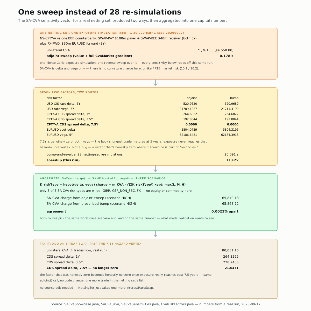
SA-CVA is delta and vega only. Unlike FRTB market risk (10.1's curvature
charge, 10.2's per-class curvature bucket), there is no curvature term
anywhere in SaCva's aggregation — not a simplification this page makes,
but the shape of the regulation itself (MAR50 has no second-order CVA
charge). One fewer shocked repricing per risk factor than 10.1 needed,
before any code runs at all.
Build the netting set
The exact book this page reprices, straight from SaCvaShowcase:
CreditName counterparty = new CreditName("CPTY-A",
    HazardCurve.fromFlatSpread(150.0, 0.40, 10.0), 0.40,
    CreditName.Rating.BBB, CreditName.Sector.FINANCIAL);

NettingSet nettingSet = new NettingSet("NS-CPTY-A", counterparty, List.of(
    InterestRateSwap.payer("SWAP-PAY", 100_000_000.0, 0.032, 5.0),
    InterestRateSwap.receiver("SWAP-REC", 40_000_000.0, 0.028, 5.0),
    new FxForward("FX-FWD", FxForward.Side.BUY_FOREIGN, 30_000_000.0, 1.10, 3.0)));
Two swaps and an FX forward, small enough to read in one screen, large enough to touch rate, credit and FX risk at once — the whole point of a netting set.
Run the exposure simulation once
ExposureSimulation prices every trade in the netting set at every date
on a Monte-Carlo grid and integrates the expected exposure against the
counterparty's hazard curve. One .run() call, with gradients enabled,
gives the value and every partial derivative in the same pass:
ExposureSimulation simulation = new ExposureSimulation(nettingSet, 20).on("cpu-jit");
CvaResult swept = simulation.run(base, paths, seed);
Real numbers, 30,000 exposure paths, seed 20260902, cpu-jit:
unilateral CVA 71,761.53 (standard error 550.80), the adjoint sweep
itself taking 0.178 s for the value and the full CvaMarket gradient
together.
Read the sensitivity vector two ways
Route B reads the seven SA-CVA factors straight off that one gradient.
Route A is the letter-compliant fallback: shock each factor and
re-simulate, using a Richardson-extrapolated central difference (steps
h and 2h, four re-simulations per factor) so the finite difference
clears floating-point round-off before comparing it to the sweep:
Sensitivities adjoint = SaCvaSensitivities.adjoint(swept, keys);
SaCvaSensitivities.BumpResult bump =
    SaCvaSensitivities.bumpAndRevalue(simulation, base, paths, seed, keys);
| risk factor | adjoint | bump |
|---|---|---|
| USD OIS rate delta, 5Y | 520.9620 | 520.9689 |
| USD rate vega, 5Y | 21709.1227 | 21711.3190 |
| CPTY-A CDS spread delta, 1Y | 264.6822 | 264.6822 |
| CPTY-A CDS spread delta, 3.5Y | 192.8044 | 192.8044 |
| CPTY-A CDS spread delta, 7.5Y | 0.0000 | 0.0000 |
| EURUSD spot delta | 5804.0739 | 5804.3196 |
| EURUSD vega, 5Y | 62186.6481 | 62184.3918 |
Seven factors, four evaluations each on Route A: 28 netting-set
re-simulations, 20.091 s, against Route B's one sweep, 0.178 s —
113.2× this run. (Take the exact multiple with a grain of salt: it's a
cold run, and it moves around from one run to the next depending on how
warmed-up the JIT already is — the shape, O(1) against 4N, is the
part that doesn't.)
The 7.5-year CDS spread delta comes back exactly 0.0000, both routes,
and that's not a coincidence or a bug: CvaRiskFactors fixes the
credit-spread tenor grid at {1.0, 3.5, 7.5} years, but this netting
set's longest trade — either 5-year swap — is the last date the exposure
simulation ever touches. The counterparty's default probability beyond
five years genuinely never enters this book's CVA, so its derivative is
honestly zero on both the sweep and the bump. A sensitivity vector that
agrees on a real zero is still a reconciliation, not a coincidence.
Aggregate into a capital charge
SaCva.charge reuses the exact NestedAggregation class Chapter 9 built
and 10.1/10.2 already leaned on — a risk type's charge is hypot(delta, vega), risk types combine as a sum of squares scaled by the supervisory
multiplier m_CVA, and the whole thing runs three times, one per
correlation scenario, keeping the largest:
double kRiskType = Math.hypot(delta, vega);
sumOfSquares += kRiskType * kRiskType;
// ...
perScenario.put(scenario, parameters.mCva() * Math.sqrt(sumOfSquares));
Only three of the regulation's five SA-CVA risk types are wired into
SaCva.RISK_TYPES — GIRR, CSR_NON_SEC, FX — because this book has
no equity or commodity exposure to aggregate; the array is hardcoded to
what this demo needs, not padded out to all five.
Both routes, scenario HIGH in both cases: from the adjoint sweep,
65,870.13; from the prescribed bump, 65,868.72 — 0.0021% apart.
That agreement, not either number alone, is what a model-validation team
actually wants to see before trusting the fast route.
Try it yourself
The 7.5-year factor is zero only because nothing in the book reaches that
far. Add a fourth trade, InterestRateSwap.payer("SWAP-LONG", 20_000_000.0, 0.033, 8.0), to nettingSet's trade list and rerun — no other code
change needed. Real numbers from doing exactly that: CVA rises to
80,031.16, the 1-year and 3.5-year CDS deltas shift a little
(264.3265, 220.7405), and the 7.5-year one wakes up: 21.0471,
no longer zero. Same adjoint() call, same tape shape — the only thing
that changed is what the book's exposure actually reaches.
▶️ Run it
The same netting set, live: one adjoint sweep against the seven-factor
prescribed bump — right here, on a stand-in for the real
ExposureSimulation rewritten around chapter 1.3's cell's own limitation,
rec.input() directly instead of Nabla.Inputs<CvaMarket>'s reflection
layer. SaCva and SaCvaSensitivities.adjoint run completely unmodified:
Or run the real thing:
mvn -o -q install
mvn -o -q -pl nablatensor-examples exec:java \
  -Dexec.mainClass=com.nablatensor.examples.SaCvaShowcase
Defaults to cpu-jit, 30,000 exposure paths, no GPU. -Dpaths= overrides
the path count if you want to watch the bump-vs-adjoint gap widen or
narrow with precision.
⚠️ What this doesn't do
One netting set, one counterparty, no collateral agreement — the smallest
book that touches rate, credit and FX risk at once.
CvaShowcase.java
is the portfolio-scale companion: two netting sets against two
counterparties (one under a daily-margined collateral agreement),
aggregated into one SA-CVA charge, plus BA-CVA in both its reduced and
full forms and the three PRA standardised methods — none of that runs
here. SaCvaParameters.demo()'s risk weights, correlations and m_CVA
are explicitly indicative, same as every parameter table this chapter has
used since 10.1; the EAD proxy behind the wider CVA-risk framework is
alpha × EPE rather than a full SA-CCR/IMM calculation, and wrong-way
risk beyond that multiplier is out of scope.
What's next
→ Deeper: SA-CVA, from the regulation to the code walks the same reconciliation with more benchmark detail — cold-vs-warm timing, the full narrated terminal session, and why the gap is wider here than for a single option's Greeks. → Next: ISDA SIMM: how banks agree on initial margin without a regulator in the room — the same sensitivities, grouped a new way, plus a concentration factor FRTB never needed.