Supervisory stress testing
One long call, one short put, revalued on a 3-scenario-by-4-horizon grid — the same recorded kernel replayed 12 times, never rebuilt. The worst projected loss lands at the nearest horizon, not the furthest one, and a naked call shows the reader why: there's simply less optionality left to lose the longer you wait.
A regulator asks every big bank the same question once a year: if the economy turns severely adverse, how much does your book lose, one quarter at a time, for the next three? Answering that for one position means full-revaluing it at every point on a scenario-by-horizon grid. Answering it for a real bank's book means doing that thousands of times over — and none of it needs a second recording of the kernel.
The whole story
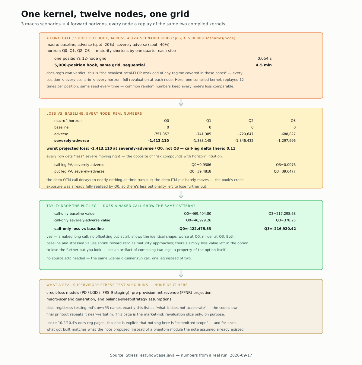
docs-reg/stress-testing.md calls this "the heaviest total-FLOP workload
of any regime covered in these notes" — heavier than FRTB, SA-CVA, or
SIMM, because it multiplies every position by every macro scenario by
every forward horizon, full revaluation at each node. This page's own
number for a 5,000-position book, run sequentially on cpu-jit: 4.5
minutes — every node still the same recorded kernel, replayed under a
moved market, never rebuilt.
Build the grid
Three macro scenarios, four horizons, crossed into twelve named nodes:
List<Scenario> macro = List.of(
    Scenario.of("baseline"),
    Scenario.of("adverse",
        Shock.relative("spot", -0.20), Shock.additive("vol", 0.05), Shock.additive("rate", -0.0075)),
    Scenario.of("severely-adverse",
        Shock.relative("spot", -0.40), Shock.additive("vol", 0.15), Shock.additive("rate", -0.015)));

List<Scenario> horizons = List.of(
    Scenario.of("Q0", Shock.additive("maturity", 0.00)),
    Scenario.of("Q1", Shock.additive("maturity", -0.25)),
    Scenario.of("Q2", Shock.additive("maturity", -0.50)),
    Scenario.of("Q3", Shock.additive("maturity", -0.75)));
Each horizon shock shortens the option's remaining maturity by another
quarter — this is 9.3's own Scenario/Shock DSL, just crossed two ways
instead of listed flat, the same "declare the shocks as data" idea 10.1
already used for two shocks instead of eight.
Revalue the book, every node
The book is a long call plus a short put on the same underlying — so a crash hurts both legs at once, the way a real book's losses compound:
Map<String, Nabla.TypedValuation<EquityMarket>> callPv =
    ScenarioRunner.run(callPricer, market, grid, scenarios, seed);
Map<String, Nabla.TypedValuation<EquityMarket>> putPv =
    ScenarioRunner.run(putPricer, market, grid, scenarios, seed);
Real numbers, 500,000 scenarios per node, cpu-jit, seed 42 — loss
versus baseline at every node:
| macro \ horizon | Q0 | Q1 | Q2 | Q3 |
|---|---|---|---|---|
| baseline | 0 | 0 | 0 | 0 |
| adverse | -757,357 | -741,385 | -720,647 | -688,827 |
| severely-adverse | -1,413,110 | -1,383,145 | -1,346,432 | -1,297,996 |
The worst projected loss is -1,413,110, at severely-adverse / Q0 —
the nearest horizon, not the furthest one. The call-leg delta there,
read off the same grid replay with no second risk run: 0.11.
Every row above gets less severe moving right, the opposite of "risk
compounds with time" intuition. The per-leg prices under
severely-adverse explain why: the call, now deep out of the money after
a 40% crash, decays from 0.9386 at Q0 to 0.0076 at Q3 — running
out of time only makes recovery less likely. The put, deep in the money
after the same crash, barely moves (39.4818 to 39.6477). The book's
crash exposure is already fully realized at Q0; there's nothing left
for the horizon axis to add.
Try it yourself
Is that shape special to combining a call and a put, or does a naked call
alone show it too? Rerun the same ScenarioRunner.run call with the put
leg dropped entirely. Real numbers: the call-only baseline value falls
from 469,404.80 (Q0) to 217,298.68 (Q3) from time decay alone;
under severely-adverse it falls from 46,929.26 to 378.25. The loss
versus baseline: -422,475.53 at Q0, only -216,920.42 at Q3 — the
same pattern, worse near, milder far, with no put leg anywhere in sight.
It's a property of the option running low on time, not an artifact of
netting two legs together.
▶️ Run it
The same grid, live: two compiled kernels, twelve named nodes, never
rebuilt — right here, built directly on setInput per node instead
of MonteCarlo/Nabla.Pricer's reflection layer, the same point 9.3's
cell made about ScenarioRunner:
Or run the real thing:
mvn -o -q install
mvn -o -q -pl nablatensor-examples exec:java \
  -Dexec.mainClass=com.nablatensor.examples.StressTestShowcase
Defaults to cpu-jit, 500,000 scenarios per node, no GPU.
⚠️ What this doesn't do
docs-reg/stress-testing.md's own §3 names exactly what a pricing engine
doesn't accelerate, and the showcase's own final printout repeats the
same list almost verbatim: credit-loss models (PD/LGD, IFRS 9 staging),
pre-provision net revenue (PPNR) projection, macro-scenario generation,
and balance-sheet-strategy assumptions. This page is the market-risk
revaluation slice only, on purpose — the part a full supervisory stress
test spends most of its compute on, not the part that decides what "how
bad" means economically.
Worth noting for once, rather than flagging a gap: unlike 10.2's
frtb-sa.md and 10.4's isda-simm.md, this doc never claims a dedicated
package already exists — its own header says "Not committed scope." What
got built (StressTestShowcase, tagged in ExamplesSmokeTest) matches
what the note proposed, reusing com.nablatensor.scenario.* directly, no
phantom module this time.
What's next
→ Deeper: docs-reg/stress-testing.md
covers the real programme cadences (EBA/ECB, Fed DFAST/CCAR, BoE/PRA) and
why this is called the headline "27h → 11min" workload.
→ Next: Climate scenario analysis —
this exact harness, unchanged, fed a 25-year horizon and a different
scenario set, with an intuitive result instead of this page's
counterintuitive one.