FRTB curvature, explained simply

You're about to ask an options book the question a regulator asks every bank: how badly can this position lose money if the market jumps 30% in either direction? The expensive part is repricing the option twice, once in each shocked market. Everything after that is a few lines of arithmetic.

The whole story

Did you know?

ScenarioRunner.run(mc, base, shocks, scenarios, seed) takes exactly one seed for the whole scenario set — base, up, and down all draw from it in the same loop. That's not a convention the demo happens to follow; it's the only way to call the method. If the three markets used different random paths, part of the difference between them would be Monte-Carlo noise, not curvature — this is the textbook "common random numbers" variance-reduction trick, enforced by the signature rather than left to the caller's discipline.

Create the market and the shocks

The setup is a MonteCarlo build you've already seen, plus a ScenarioSet of three named markets:

EquityMarket market = EquityMarket.atmOneYear();

ScenarioSet shocks = ScenarioSet.list(
    Scenario.of("base"),
    Scenario.of("spot-up", Shock.relative("spot", 0.30)),
    Scenario.of("spot-down", Shock.relative("spot", -0.30)));

atmOneYear() is 3.1's own market again: spot 100, strike 100, vol 20%, rate 3%, maturity one year. The three Scenario objects are only data — "don't move spot," "multiply spot by 1.30," "multiply spot by 0.70" — they don't touch a kernel until ScenarioRunner runs them.

Calculate delta once

A .greeks() kernel gives delta from one adjoint reverse sweep, exactly the way 1.3 and 2.2 already used it — no bump, no second market:

MonteCarlo.of(Products.asianCall())
    .market(market).steps(252).fp64().greeks().on("cpu-jit").build();

The position is short, so the demo negates both the price and delta it gets back.

Reprice the large shocks

This is the expensive stage. A second, price-only kernel replays for the base, up, and down markets — compiled once, never rebuilt for a shock:

ScenarioRunner.run(pricer, market, shocks, scenarios, seed);

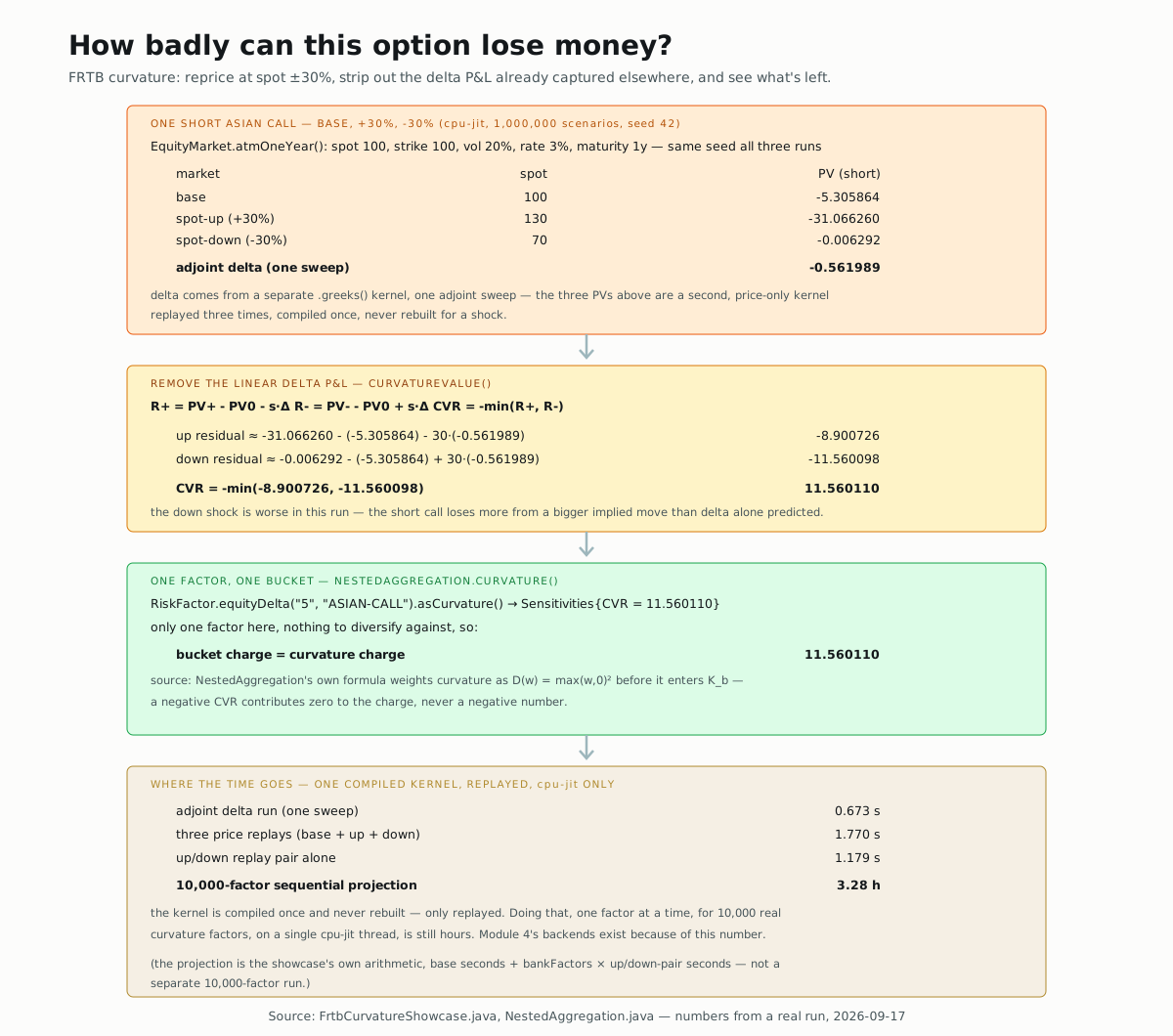
Ran it for real, 1,000,000 scenarios, 252 fixings, cpu-jit, seed 42:

market	spot	PV (short)
base	100	-5.305864
spot-up	130	-31.066260
spot-down	70	-0.006292
adjoint delta (one sweep)		-0.561989

Did you know?

The showcase itself computes the number that motivates this whole section: it times the up/down replay pair (1.179 s here), multiplies by a bank-scale 10,000 factors, and adds the base valuation. On this machine, on cpu-jit, sequentially repricing 10,000 real curvature risk factors this way — one after another, on one thread, with the kernel compiled exactly once and never rebuilt — projects to 3.28 hours. That's the whole reason Chapter 4's other five backends exist: not because cpu-jit is slow at any one repricing, but because a real bank book has thousands of factors and only one overnight batch window to price all of them.

Remove the ordinary delta effect

FRTB curvature wants the bending of the price, not the straight-line move delta already explains. curvatureValue computes:

static double curvatureValue(double pvBase, double pvUp, double pvDown,
                             double shock, double delta) {
  double upNonLinear = pvUp - pvBase - shock * delta;
  double downNonLinear = pvDown - pvBase + shock * delta;
  return -Math.min(upNonLinear, downNonLinear);
}

With the real numbers above (shock = 0.30 × 100 = 30):

up residual   ≈ -31.066260 - (-5.305864) - 30·(-0.561989) = -8.900726
down residual ≈  -0.006292 - (-5.305864) + 30·(-0.561989) = -11.560098

CVR = -min(-8.900726, -11.560098) = 11.560110

The down shock is worse in this run — the short call loses more from a 30% drop than its own delta predicted, and that gap is exactly what curvature is meant to capture.

Put CVR into an FRTB bucket

RiskFactor factor = RiskFactor.equityDelta("5", "ASIAN-CALL").asCurvature();
Sensitivities curvature = Sensitivities.builder().add(factor, cvr).build();
double charge = NestedAggregation.curvature(
    (left, right) -> left.equals(right) ? 1.0 : 0.25,
    (left, right) -> left.equals(right) ? 1.0 : 0.15)
    .aggregate(curvature).total();

"5" is the example's equity bucket, "ASIAN-CALL" names the factor, and asCurvature() tags the number as CVR rather than delta. With one factor in one bucket, there's nothing to diversify against, so the bucket charge and the curvature charge are the same number: 11.560110.

NestedAggregation's own doc comment gives the formula a plain delta factor doesn't get: curvature weights each factor as D(w) = max(w,0)² before it enters the bucket's risk number, not w². A negative CVR — a shock that happens to help the position — contributes exactly zero to the charge. It never earns a capital credit, and it never turns into a negative number either.

Try it yourself

SHORT_POSITION is a private constant, -1.0. Flip it to 1.0 (the same option, held long instead of sold) and rerun. The base PV and delta both flip sign, and so does the shape of the worse residual — CVR comes out negative this time. Before you assume that shrinks the charge, check what D(w) = max(w,0)² from the section above actually does to a negative weighted sensitivity, and predict the charge before you look at what the program prints.

▶️ Run it

The same repricing, live: one compiled kernel, three named spots — right here, in the interactive example, on the cpu engine directly instead of cpu-jit, for the reflection reason 1.3's cell already established. NestedAggregation runs completely unmodified — it's the same real class 9.4 already used:

Or run the real thing:

mvn -o -q install
mvn -o -q -pl nablatensor-examples exec:java \
  -Dexec.mainClass=com.nablatensor.examples.FrtbCurvatureShowcase \
  -Dscenarios=10000 -Dsteps=252

Defaults to cpu-jit, no GPU backend touched. The colorful version of the same demo — same math, a walkthrough narration on top — is ./demo/frtb-curvature-on-cuda.sh, which does use CUDA; run it only if you have an NVIDIA GPU and want that backend, not as part of this page.

⚠️ What this doesn't do

This is a focused showcase of one FRTB equity curvature factor, from input to charge. It is not a complete FRTB implementation. Missing, on purpose: the other six FRTB risk classes; regulatory parameter tables for every bucket; delta and vega capital aggregation; default risk charge or the residual risk add-on; and any trade netting, market-data loading, or regulatory sign-off. Chapter 10.2 picks up delta and vega capital — the rest of the standardised approach beyond curvature.

What's next

→ Deeper: FRTB curvature showcase covers the full backend comparison (scalar, JIT, SIMD, and GPU replay times) and the exact configuration knobs this page kept fixed. → Next: FRTB standardised approach, the rest of it — delta and vega capital, DRC, RRAO, and the max-per-class rule that keeps none of it from diversifying against the rest.