SA-CVA, from the regulation to the code

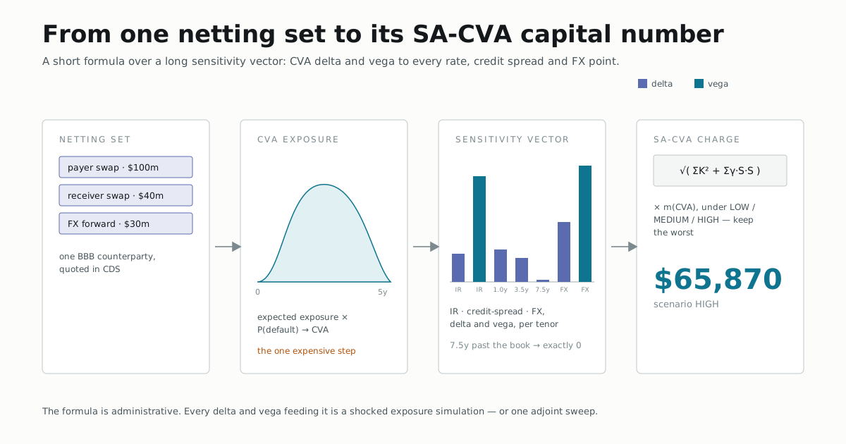
If you've gone looking for a practical, code-level walkthrough of SA-CVA — the standardized approach to CVA capital under Basel III / CRR3 — what you mostly find is the regulation text itself (MAR50 / CRR3 Article 383) or a vendor's sales page. Both assume you already have the hard part: a sensitivity vector for your netting set, broken out by risk type, bucket and tenor, computed under three prescribed correlation scenarios. Getting that vector is most of the actual engineering work, and it's the part nobody shows.

What SA-CVA actually asks for

The formula itself, once you have the inputs, is almost administrative. For each risk type — interest rate, credit spread, FX, equity, commodity — you aggregate delta and vega sensitivities within buckets, combine buckets with a prescribed correlation, and get a risk-type capital number K:

double kRiskType = Math.hypot(delta, vega);

The risk types combine as a sum of squares, scaled by the supervisory multiplier m_CVA, and the whole thing is computed three times — once per correlation scenario (LOW, MEDIUM, HIGH) — keeping whichever is largest. That's SaCva.charge(...) in about forty lines. The regulation is precise about this part and the code mirrors it closely.

The expensive part: getting the sensitivity vector

CVA itself is already a nested Monte-Carlo problem — you simulate the underlying market, revalue every trade in the netting set at every future date, and integrate the expected positive exposure against the counterparty's default probability. A SA-CVA sensitivity vector asks for the derivative of that number with respect to every rate, credit-spread and FX input the desk is exposed to.

The letter-compliant way to get a derivative when you don't have one analytically is the same bump-and-revalue from the previous post: shock one risk factor, re-run the entire netting-set exposure simulation, shock it back the other way, take the difference. Done carefully it's a little more than that — each factor's slope here is a Richardson-extrapolated central difference: two-sided differences at step h and at 2h, four re-simulations per factor. The extra pair of points cancels the O(h²) term and leaves O(h⁴) error, which lifts the finite difference clear of the floating-point round-off floor so it still reconciles with the adjoint sweep. For a book with N risk factors that's 4N re-simulations — and unlike a single option's Greeks, here each one is itself a full nested Monte-Carlo exposure calculation, not a cheap repricing.

We built a small, realistic netting set and ran it both ways:

CreditName counterparty = new CreditName("CPTY-A",
    HazardCurve.fromFlatSpread(150.0, 0.40, 10.0), 0.40,
    CreditName.Rating.BBB, CreditName.Sector.FINANCIAL);

NettingSet nettingSet = new NettingSet("NS-CPTY-A", counterparty, List.of(
    InterestRateSwap.payer("SWAP-PAY", 100_000_000.0, 0.032, 5.0),
    InterestRateSwap.receiver("SWAP-REC", 40_000_000.0, 0.028, 5.0),
    new FxForward("FX-FWD", FxForward.Side.BUY_FOREIGN, 30_000_000.0, 1.10, 3.0)));

Two interest-rate swaps and an FX forward against one BBB counterparty — small enough to read in full, large enough to touch interest-rate, credit and FX risk simultaneously, which is exactly the point of a netting set.

Two routes, one book, run live

Route A, the prescribed bump: re-simulate the whole netting set's exposure once per shocked risk factor, central-difference the CVA. Route B, the adjoint sweep: run the exposure simulation once, and read every sensitivity off a single reverse pass over the same tape. We ran both, on referential machine, right before publishing:

$ mvn -o -q -pl nablatensor-examples exec:java \
    -Dexec.mainClass=com.nablatensor.examples.SaCvaShowcase

Netting set NS-CPTY-A: 2 interest-rate swaps + 1 FX forward, one BBB counterparty
30,000 exposure paths, seed 20260902, engine cpu-jit

unilateral CVA           71,761.53  (se 550.80)
adjoint sweep            0.144 s  (value + full CvaMarket gradient)

risk factor                               adjoint           bump
USD OIS rate delta, 5Y                   520.9620       520.9689
USD rate vega, 5Y                      21709.1227     21711.3190
CPTY-A CDS spread delta, 1Y              264.6822       264.6822
CPTY-A CDS spread delta, 3.5Y            192.8044       192.8044
CPTY-A CDS spread delta, 7.5Y              0.0000         0.0000
EURUSD spot delta                       5804.0739      5804.3196
EURUSD vega, 5Y                        62186.6481     62184.3918

bump-and-revalue         28 netting-set re-simulations, 39.061 s
speedup                  270.8x

SA-CVA charge  from adjoint sweep   65,870.13  (scenario HIGH)
SA-CVA charge  from prescribed bump 65,868.72  (scenario HIGH)

Seven risk factors, twenty-eight re-simulations for the bump vector; one forward pass and one reverse sweep for the adjoint vector. Take the 271x in that block with salt — it's a cold run, and it swings between roughly 150x and 350x from one run to the next. The sweep is JIT-compiled and warm almost immediately; the twenty-eight bump re-simulations are still paying compilation cost while they're being timed. The narrated session below — warm after four earlier stages, and on 200,000 paths — is the steadier picture: about 28 s of bump against a 1 s sweep, call it 25–30x. What doesn't depend on warm-up or path count is the shape — O(1) against 4N — and the reconciliation: both routes pick the same worst-case correlation scenario (HIGH) and land on the same capital number to within 0.003%, which is exactly what a regulator or an internal model-validation team would want to see before trusting the faster method.

One row is worth a second look: the 7.5-year CDS tenor comes back exactly zero both ways. That's not a bug — the netting set's longest trade matures at five years, so the counterparty's default probability beyond five years never touches this book's exposure. A sensitivity vector that's honestly zero where it should be zero is part of what "reconciles" means here.

If you'd rather watch it than read it, here is the same calculation on cpu-jit as a narrated session — on a netting set of the same shape (two swaps and an FX forward against one BBB counterparty), the CDS quotes stripped to a hazard curve, the Monte-Carlo exposure simulation, then the full risk vector both ways, reconciled factor by factor. It runs on past the SA-CVA charge into BA-CVA and the three PRA methods, which this article doesn't cover.

Why the gap is wider than for vanilla Greeks

The bump-vs-adjoint post found roughly 8–10x on plain vanilla and exotic equity Greeks. SA-CVA opens that gap wider, for two compounding reasons:

• More factors, and each one costs four passes. Five equity Greeks by central difference is eleven replays. Seven SA-CVA risk factors, each a Richardson-extrapolated slope, is 4N — twenty-eight. The bump side scales linearly in risk factors; the sweep doesn't scale at all, so the gap widens with every factor you add.
• A far more expensive base case. A CVA exposure simulation is Monte-Carlo-inside-Monte-Carlo — exposures on a time grid, integrated against a hazard curve — not a single terminal payoff. Every one of those twenty-eight re-simulations pays that full cost again; the adjoint sweep pays it once, no matter how many risk factors come off the back of it.

That second point is the actual argument for adjoint AD in an XVA desk specifically, more than in a single-product Greeks desk: the more expensive the base valuation, the more a bump loop's O(N) re-simulations cost, and the more a sweep's O(1) gradient is worth.

What this example leaves out — and where the rest is

The run above is deliberately the smallest thing that makes the point: one netting set, one counterparty, no collateral agreement, and the interest-rate, credit-spread and FX risk types. SA-CVA itself is only ever delta and vega — there is no curvature charge in it, unlike FRTB market risk — so that isn't missing, it doesn't exist.

What is left out here is the portfolio around the single netting set. CvaShowcase.java in nablatensor-examples is the fuller version, and it runs the same way (mvn -q -o -pl nablatensor-examples exec:java -Dexec.mainClass=com.nablatensor.examples.CvaShowcase):

• Two netting sets against two counterparties, aggregated into one SA-CVA charge under the three correlation scenarios.
• A collateral agreement — the second netting set sits under a daily-margined CSA with a threshold and a margin period of risk, so its exposure is the collateralised profile, not the raw netted mark-to-market.
• BA-CVA in both its reduced (closed-form) and full (single-name-CDS-hedge recognition) forms, and the three PRA standardised methods with the binding charge picked out.

Both examples are wired into the nablatensor-examples smoke tests, so a mvn -o test that stays green is the guarantee these numbers still reproduce.

The reconciliation earlier is still the piece worth trusting first: that the sensitivity vector a real capital calculation needs can come from one sweep instead of four re-simulations per factor, on a real (if small) book, with the numbers to prove it agrees.