Your first Jit.compile

The same calculation, fresh numbers

You need to evaluate -(x² + 3) repeatedly. On [1, 2, 3], the answer is [-4, -7, -12]. On [-1, 0, 4], it is [-4, -3, -19]. The arithmetic stays the same; only the input values change. This is a small, useful place to separate describing a tensor calculation from replaying its execution plan.

Jit.compile creates a callable object. Its first call for an input signature captures the tensor operations and returns their result. Compatible later calls replay the stored plan with their own input buffers. A signature describes the input's shape, dtype, device and backend. The actual numerical values remain runtime inputs.

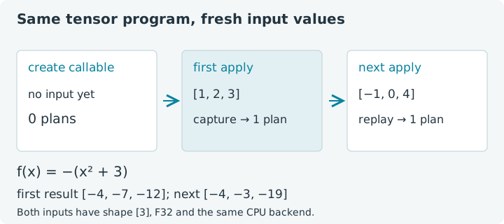
Choose Run all, then change individual inputs. The cells share an explicitly typed compiled-function variable in one Java session. This notebook uses the bundled jax4j 0.2.1 CPU backend. The browser JVM is emulated, so the examples teach semantics and cache behavior rather than native performance. Leaving or reloading the page discards edits, plans and session state.

1. Create the callable before supplying data

The lambda describes a square, scalar addition and negation. Its intermediate tensors are created through JIT's tracing backend, which manages them while building and executing the plan. We own the ordinary tensors passed in and the new output tensors returned from these examples.

Creating the callable alone does not capture an input-dependent plan. There is no input shape yet. Check that its cache starts empty.

Expect plans before input: 0. The compiled object implements UnaryOperator<Tensor>, so .apply(input) is the entry point you will use repeatedly. It is a jax4j tensor-program abstraction; the capture process records backend operations reached by the Java lambda.

Try this: change 3 to 5 and rerun setup. You have created a different compiled object with an empty cache. Its first answer on [1, 2, 3] will be [-6, -9, -14]. Restore 3 and rerun setup before following the reference cache counts below. Editing text alone does not execute the modified cell.

2. The first application captures and computes

The first input has shape [3]. The capture runs the Java body, records the calculation through the tracing backend and produces an output. You do not need a separate invocation to get the first numerical result.

Expect [-4, -7, -12] and one cached plan. blockUntilReady() is an explicit completion point, useful when reasoning about asynchronous devices. The later .toFloatArray() also needs a host-visible result. Neither call belongs inside the compiled lambda in these examples; reporting happens after the tensor computation has returned.

The eligible elementwise chain can be fused by the backend rather than launched operation by operation. Matrix products, reductions and other operations introduce their own execution boundaries. The existence of one cached plan does not tell you how many kernels it contains, nor guarantee a speedup on every backend or problem size.

3. New values reuse the same signature

The second input is a fresh tensor with different values but the same shape and placement. Those new values must influence the answer. Replaying a plan reuses the calculation, not the previous output numbers.

Expect [-4, -3, -19] and still one plan. Change the input to [2, 4, 6] and predict [-7, -19, -39]. The compiled function can outlive each of these individual input and output tensors. Once their use is complete, the try blocks close them; the next call supplies a fresh input handle.

The function is elementwise, so changing only one entry affects only the corresponding output entry. This makes a good first check when experimenting: keep the shape fixed, alter one recognizable number and confirm which output changes. A function involving a reduction or matrix product would connect positions differently, even with the same capture-and-replay mechanism.

4. A different shape creates another plan

A four-element input has another signature. This compiled object keeps a separate plan for it, and the Java body is captured for that new case. Returning to a previously seen signature can then reuse its original plan.

Expect [-4, -7, -12, -19] and two plans when running from the top. Rerunning this cell with the same shape does not add a third plan. Try five entries with shape [5], then return to four. Watch the count alongside the results so you can distinguish new numerical data from a new specialization.

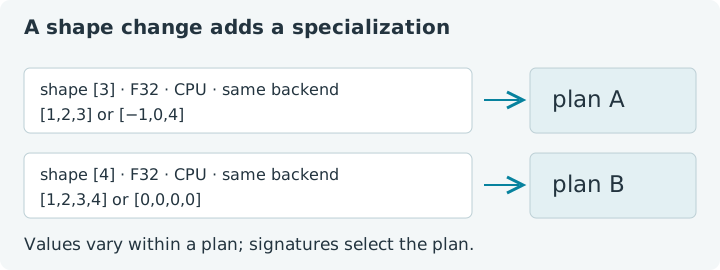
Cache counts are cumulative for this compiled object. Restarting the kernel or rerunning setup creates fresh state. If your count differs from the printed reference after an experiment, first ask which signatures that particular object has already seen. A notebook's execution history is part of the experiment, not an invisible reset between cells.

5. Revisit the first signature

We can now call the three-element case again. The values are different from both earlier three-element inputs, but the signature is familiar.

Expect [-3, -3, -3] and two plans in the unmodified sequence. The same array of six numbers could also be reshaped to [2, 3] or [3, 2]; those would be distinct signatures despite sharing the same element count. Predict the output shape for each, then try one by adding explicit dimensions to Tensors.array.

For this version, the compiled object exposes a plan count but no public cache clear or eviction control. Avoid feeding an unbounded variety of shapes into one long-lived callable without considering retained plans. Creating a new callable starts another cache; ordinary Java reachability then governs the old object's lifetime. A new plan is not itself evidence of an error.

6. Compile a derivative function too

The gradient from Chapter 2 is another tensor-to-tensor function. We can compose it with compilation. For sum(x²), the gradient is 2x, so [1, 2, 3] should produce [2, 4, 6]. This example keeps the calculation small enough to inspect without mixing in an optimizer or a training loop.

Try [-1, 0, 4], giving [-2, 0, 8]. This separate compiled object has its own cache; it does not share the polynomial object's plan count. The transform composition still needs derivative rules for every operation it encounters. Compilation does not make an unsupported derivative available.

Jit.apply is also available for a one-shot traced execution. The persistent object returned by Jit.compile adds reusable execution plans per signature. Keep that distinction in mind when reading examples that use the shorter one-shot form.

Continue with capture rules, cache keys and host reads before closing over mutable Java configuration. Revisit scalar gradients if you want to change the final loss and predict the compiled derivative.