Capture rules, cache keys and host reads

Change the bias, keep the old answer?

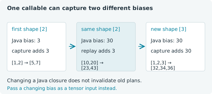
A compiled function computes 2x + bias, and the Java array holding bias initially contains 3. Capture it for shape [2], change the Java bias to 30, and call the same shape again. The cached plan still adds 3. Now call shape [3]: that new capture sees 30. One compiled object can therefore contain plans built under different Java-side configuration.

This is a deliberately constructed example of capture-time behavior. It is useful to see the mechanism once, then write production functions with explicit runtime tensor inputs and stable configuration. A tiny side-effect counter will show exactly when the Java body runs.

Choose Run all for the documented sequence, then experiment with the cell order. This notebook uses jax4j 0.2.1 on the emulated CPU. Its counter and mutable Java array are teaching instruments; the tensor result should normally be determined by explicit inputs plus deliberately fixed configuration. Reloading discards edits and all state.

1. Count captures, not applications

The counter increments inside the Java body supplied to Jit.compile. The callable is created immediately, but its body runs when it needs to capture a new input signature. During compatible replay, Java statements such as this increment are not re-executed.

A one-element Java array lets us change the bias without replacing the lambda's reference to that array. The number extracted by bias[0] becomes a scalar operand in the recorded tensor calculation.

Expect zero captures. The counter deliberately makes the function impure so we can observe capture; it is not a per-call metric. Logging, random draws through ordinary Java utilities and updates to collections inside such a body have the same scheduling issue: their Java execution follows capture rather than every tensor replay.

2. Capture the first signature

Our initial input is [1, 2]. With bias 3, its output is [5, 7]. The first successful capture should leave both the counter and the cached plan count at one.

Rerun this cell without resetting setup. Its output is unchanged, and both counts stay one. Now change just the input numbers: a fresh [10, 20] should produce [23, 43]. The plan accepts runtime values even though it retains the scalar bias chosen during capture.

The input signature includes shape, dtype, device and backend. Neither the input's numerical values nor the contents of an arbitrary Java array in the closure are cache-key fields. Changing a Java object does not automatically invalidate existing plans.

3. Mutate Java configuration after capture

The next cell changes the Java bias to 30 while preserving input shape [2]. Read the input, the live Java value and the actual tensor result separately. They describe three different parts of the experiment.

Expect a live Java bias of 30, result [23, 43] and one capture. The existing plan adds the scalar value 3 recorded earlier. Try setting the bias to -100 and repeating the same shape. Its result still follows the first plan. Restore 30 before creating the next signature.

If the bias needs to change on every application, make it a tensor argument. The next lesson demonstrates this with a named parameter tree. If the bias really is fixed configuration, keep it fixed for the callable's lifetime or create a new compiled object when the configuration changes. Treating a Java closure as a dynamic argument list invites hard-to-explain results.

4. A fresh signature sees the current Java state

The three-element input has no cached plan yet. Its capture evaluates the Java body with bias 30, producing [32, 34, 36]. The earlier shape remains associated with its original scalar.

Expect two captures and two plans when running in order. Return to the second cell and its [1, 2] input: the result should still be [5, 7], even while bias[0] is 30. The count stays two. Now rerun setup and repeat the sequence in a different order. Which bias does each shape capture? You can predict every result from the capture history.

Closed-over tensors require a related ownership decision. They are captured as external buffer references and must remain alive while the plan uses them. They are not automatically converted into replaceable runtime parameters. Passing changing weights and state explicitly makes both the data dependency and the required lifetime easier to see.

5. Read results after the compiled function returns

A call to .item() or .toFloatArray() on a traced tensor asks for its contents in Java. During Jit.compile capture, that host read is rejected. Otherwise a Java condition or scalar constant could silently depend on the first input's data instead of becoming a replayable tensor operation.

The input deliberately contains one element, so the intended failure is the capture-time host read, not an attempt to extract a scalar from a larger array. A tensor-space replacement is t -> t.add(t). Try that in the cell and expect [4]; retain the try resource list so the successful output closes.

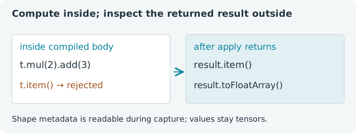
Shape metadata is different from tensor contents. Reading t.shape() during capture does not download numerical values. You can use a shape to select a Java branch or decide a fixed loop count for that specialization. The selected Java control flow is then reflected in the captured plan for that signature.

6. Branch on metadata deliberately

This function adds 100 for a two-element vector and subtracts 100 for other vector lengths. Each shape gets the branch selected at its own capture. The condition uses metadata, so the values within a fixed shape cannot change which branch is recorded.

Expect [101, 102], [-99, -98, -97] and two plans. Change the values within a while keeping length two. The first branch still applies. Restrict this particular example to vectors: it deliberately reads leading-axis length, not total element count, and does not handle a rank-zero input.

A data-dependent branch needs tensor control-flow support rather than a Java if fed by .item(). A later chapter covers those APIs. Likewise, a Java loop driven by a shape becomes a fixed recorded calculation for that shape; it is not automatically a runtime device loop.

Continue with parameter trees and structured outputs to make mutable model values explicit. Revisit your first compiled function for the basic first-capture and compatible-replay sequence.