Jacobians, Hessians and nested derivatives

When the derivative becomes the large object

A function with two inputs and three outputs has only six first derivatives. We can print all of them. A scalar loss with a million inputs has a million gradient entries, but its dense Hessian has a trillion. Before choosing a transform, decide which derivative information you actually need to store.

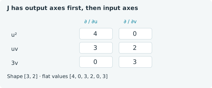
We will reuse f(u, v) = [u², uv, 3v] from the previous notebook. At [2, 3], its Jacobian has rows [4, 0], [3, 2] and [0, 3]. Each row belongs to an output; each column belongs to an input. That ordering matters when interpreting both printed arrays and matrix products.

Choose Run all, then revisit individual cells. This notebook uses jax4j 0.2.1 on the emulated CPU, with independent state from the previous lesson. Inputs and returned derivative tensors have explicit resource owners. Inside transformed lambdas, traced intermediate allocations belong to the transform's scope. Reloading or leaving the page discards edits and Java state.

1. Define the vector map and a scalar energy

Alongside the vector function, we define E(u, v) = (u + v)² + u² + v². Expanding gives 2u² + 2uv + 2v². Its gradient is [4u + 2v, 2u + 4v] and its Hessian is [[4, 2], [2, 4]]. The cross term makes the two coordinates interact. At [2, 3], the energy is 38 and the gradient is [14, 16].

These are constructed smooth polynomials, so every derivative can be checked by hand. They also avoid nonsmooth points where a chosen derivative convention would require a separate discussion.

2. Build the Jacobian by pushing basis directions

jacfwd constructs a full Jacobian with forward-mode basis sweeps. For our two-element input, those directions are [1, 0] and [0, 1]. Their JVPs are the columns [4, 3, 0] and [0, 2, 3]. The final tensor arranges the result with output dimensions first, followed by input dimensions.

Expect shape [3, 2] and flat values [4, 0, 3, 2, 0, 3]. The flat printout is row-major: it shows the first output's two input derivatives, then the second output's, then the third output's. It does not print the basis sweeps in the order they were computed.

Try this: change the point to [1, 4]. Predict rows [2, 0], [4, 1] and [0, 3]. Then change the final output from v.mul(3) to v.mul(5) in setup. Only the final row becomes [0, 5]. Restore the original function and point when comparing the remaining reference outputs.

The axis convention extends beyond vectors. If an input has shape [2, 2] and its output has shape [3], the Jacobian shape is [3, 2, 2]. Treating that automatically as an ordinary two-dimensional matrix would lose the input axis meanings. You may flatten deliberately for linear algebra, provided you keep the ordering consistent on both sides.

3. Build the same array by pulling output basis weights

jacrev constructs a full Jacobian using reverse differentiation for each output coordinate. Here it asks three questions: the gradient of output zero, then output one, then output two. Both transforms describe the same local map and use the same output-then-input axis order.

Expect the same [3, 2] shape and six entries. In jax4j 0.2.1, these transforms perform explicit basis sweeps. Forward construction uses one JVP per input coordinate; reverse construction uses one reverse pass per output coordinate, with an initial evaluation to establish the output shape. Do not read either call as a promise of one fused derivative kernel.

For many inputs and one output, a scalar gradient usually makes more sense than materializing a general Jacobian. For many outputs but only a few input directions of interest, use JVPs. Operation cost, saved intermediates and the backend also matter; counting input and output coordinates is a starting point, not a universal speed ranking.

4. Differentiate a gradient to get curvature

A Hessian contains the derivatives of a scalar objective's gradient. For our energy, its diagonal entries are 4 and its off-diagonal entries are 2. Changing one coordinate therefore changes both components of the gradient. Transforms.hessian composes a forward Jacobian with the scalar gradient.

Expect [2, 2] and [4, 2, 2, 4]. Change the point to [10, -7] and rerun. The Hessian stays the same because this energy is quadratic. Its gradient changes, but its curvature does not. To make curvature depend on the point, try t -> t.mul(t).mul(t).sum() instead. At [2, 3], that cubic's Hessian is diagonal with entries 12 and 18.

For a scalar objective on input shape [2, 2], the Hessian has shape [2, 2, 2, 2]: two copies of the input dimensions. It has sixteen entries, not four. The square growth is in the total number of input elements.

5. Ask for a Hessian-vector product directly

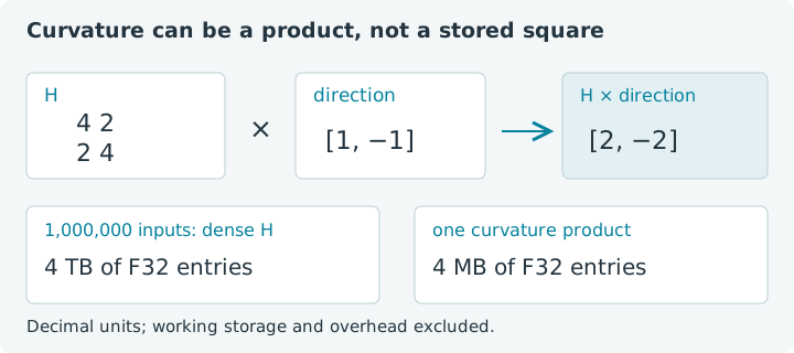
Often an algorithm needs the change of the gradient along one direction, rather than all pairwise second derivatives. Apply a JVP to the gradient function. This produces H × direction without asking the API to materialize the dense Hessian. The derivative computation still needs its own intermediates; it is not a promise of constant memory.

Expect gradient [14, 16] and product [2, -2]. Notice what value() means here: the function passed to the JVP is the gradient function, so its ordinary value is the gradient, not the original energy. Its tangent is the gradient's local change along the chosen direction.

Try direction [1, 1], giving [6, 6], then [1, 0], giving [4, 2]. Those two directions reveal different curvature. You can check each answer by multiplying the small Hessian from the previous cell by hand. The vector [1, -1] has a smaller curvature factor than [1, 1] in this example.

For a million scalar inputs, a dense F32 Hessian's entries alone occupy 1,000,000² × 4 bytes: four trillion bytes, or 4 TB in decimal units. A single million-element product has four million bytes of entries. Neither figure includes the computation's working storage or object overhead. This is a representation choice worth making before allocating the large object.

6. A nested gradient is not automatically the Hessian diagonal

The inner gradient is vector-valued. To apply grad again, we must choose a scalar reduction of that vector. Summing it asks for the gradient of the sum of all gradient components. This combines Hessian entries; it does not select just the diagonal.

Expect [6, 6], not [4, 4]. Each result sums one column of the Hessian. For this smooth scalar energy the Hessian is symmetric, so this also matches its product with the all-ones direction. The off-diagonal coupling contributes 2 to each result. A diagonal-only example could have hidden that distinction.

Replace energy with the separable cubic suggested above and predict [12, 18]. Its off-diagonal entries are zero, so the sums happen to equal the diagonal. Then differentiate that summed second derivative once more: the corresponding third-order contraction is [6, 6]. It is still a chosen contraction, not a dense three-axis third derivative tensor.

Nested transforms require derivative rules for the operations encountered at every level. Keep host reads outside transformed functions, use smooth examples when comparing higher derivatives, and treat unsupported rules as real API limits. A first derivative working does not establish that every higher order or every nonsmooth input will behave as your model intends.

Return to JVPs and VJPs when you need only products, or the scalar-loss notebook when choosing the objective. You now have three distinct questions to ask: the gradient of one score, the local change along one direction, or the full array of derivatives. Choosing among them controls both meaning and storage.