From a scalar loss to a tensor gradient

Which estimate should move, and by how much?

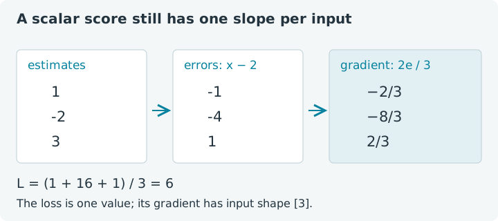
Three estimates are [1, -2, 3], and each should approach the target 2. Their errors are [-1, -4, 1]. Squaring and averaging gives a loss of 6. That one number tells us how far off the collection is, but it does not say how to change each estimate. A gradient supplies those three local sensitivities.

This is a constructed optimization problem with an answer we can see: all three estimates should become 2. Keeping the target obvious lets us inspect what differentiation does before hiding it inside a model with many parameters. The second estimate needs the largest correction; the first and third need opposite corrections of equal size.

Choose Run all, then revisit the cells and change their inputs. This notebook starts its own Java session and uses the bundled jax4j 0.2.1 CPU backend. Imports, explicitly typed declarations and the Java array persist between cells. Tensor handles inside try blocks close at the end of each block. Leaving or reloading this page discards edits and Java state.

1. Write the loss as tensor operations

Our loss is L(x) = mean((x - 2)²). The input is a three-element tensor; the output contains one value. UnaryOperator<Tensor> is Java's type for a function receiving one tensor and returning one tensor. We can pass that function to a transform instead of manually writing a separate derivative.

The lambda first creates residuals, then squares and averages them. Its intermediate tensors are allocated through the differentiation tracer and owned by the transform's temporary scope. Outside a transform, ordinary tensor expressions still need the resource ownership discussed in Chapter 0.

Expect approximately [-0.666667, -2.666667, 0.666667]. Each component is 2 × (estimate - target) / 3. Negative means increasing that estimate locally reduces the loss; positive means decreasing it does. The gradient has the same shape as the input, even though the loss has only one element.

Try this: change the second estimate from -2 to 2, then rerun setup. Its gradient becomes zero because it already matches the target. Restore the original array before comparing the following reference answers. Do not infer that every zero gradient proves a global optimum: that conclusion happens to hold for each coordinate of this simple quadratic.

2. Get the value and derivative together

Often you want both the current loss for reporting and its gradient for an update. valueAndGrad returns both from one transform invocation. Its result record is a container, not an AutoCloseable resource. Close its two tensors explicitly, as the next cell does.

The original inputs give loss 6 and gradient shape [3]. The .item() call reads the completed loss back into Java. It belongs outside the transformed function. Calling .item() or .toFloatArray() on a traced value inside the lambda attempts a host read, which this differentiation API rejects. Keep the calculation in tensor operations until the transform returns.

Automatic differentiation applies derivative rules to the operations actually executed. It does not perturb each input to estimate a slope, and it does not parse Java into symbolic algebra. The chain rule connects the local rules for subtraction, multiplication and reduction. If an operation lacks a derivative rule, the transform reports an unsupported operation; do not assume every available tensor method is differentiable.

3. Use the gradient for one update

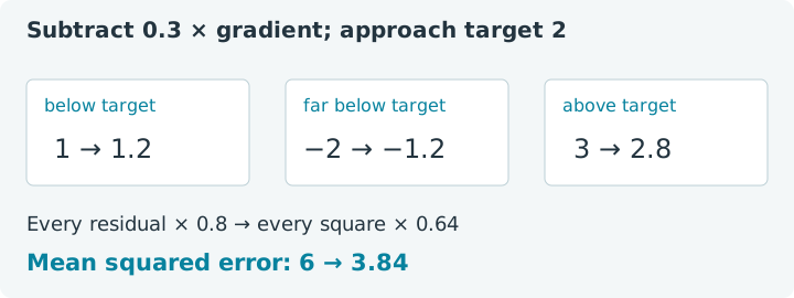
Gradient descent subtracts a scaled gradient: next = x - rate × gradient. The rate is our choice. With rate 0.3, the initial estimates become approximately [1.2, -1.2, 2.8]. Each residual shrinks to eighty percent of its old value, so the squared loss shrinks to sixty-four percent: 3.84.

Try rate 1.5. For this particular loss it reaches the target in one step. Now try 3: the residuals reverse sign without shrinking, so the loss stays at 6. A still larger rate increases it. Those outcomes come from the exact quadratic in this notebook; real models do not generally have a single rate that lands on their optimum immediately.

Change one estimate and predict its next value before running the update. The other two estimates are unaffected here because the loss adds independent squared errors. Later, a shared model parameter can influence many observations, and those contributions accumulate into that parameter's gradient.

4. The reduction is part of the model

A sum of squared errors and a mean of squared errors have the same minimizer in this example. Their gradients differ by the number of entries. Replacing mean() with sum() multiplies every gradient component by three. That changes the effect of a fixed learning rate, so a reduction is more than a reporting preference.

Expect [-2, -8, 2]. If you replace the mean loss with the sum loss in the update cell, which rate reproduces the original step? It is 0.1: divide the rate by three to compensate for the gradient's scaling. With a changing batch size, forgetting this relationship can make an otherwise sensible update behave differently.

5. A gradient needs a scalar objective

An unreduced vector of squared errors is useful, but it does not define one gradient of a scalar objective. Which output should count, and with what weight? grad requires an output containing exactly one element. In this API, a one-element shape such as [1] qualifies; it need not have rank zero. The next cell catches a deliberate missing-reduction error.

Add .sum() after t.mul(t) and rerun. The function becomes a scalar objective and its gradient becomes [2, -4, 6]. Alternatively, keep the vector output and ask a directional or weighted-output question using the JVP and VJP transforms in the next lesson. Reducing everything indiscriminately can erase the distinction you meant to study.

6. Check a slope independently

A small finite difference is a useful diagnostic for a smooth function. Here we move only the first estimate by a small amount and compare the change in loss against its analytic gradient component. This last cell uses ordinary Java arithmetic so its reference calculation is independent of the transform.

With the original array, both numbers are approximately -0.666667. The constant 17 is the other two squared errors, 16 + 1; update it if you change those estimates. It cancels in the difference, but keeping the actual objective visible makes the check easier to audit.

This quadratic has no truncation error in its central-difference slope in exact arithmetic. Rounding can still matter. For general smooth functions, a finite step introduces approximation error, while an extremely small step can lose precision through subtraction. Agreement on one input also does not validate every branch or nondifferentiable point in a larger function.

Continue with JVPs and VJPs to ask how a whole vector output changes. Revisit reductions if the distinction between preserving axes and producing one objective still feels slippery.