Measure compilation, execution and transfers

A stopwatch can time the wrong thing very precisely

A GPU operation may return a handle before its queue finishes. A first compiled call may capture a program before replay is possible. A readback may move data and allocate a Java array. If all three appear under one number called “execution,” that number is hard to explain or reproduce.

We will measure x² + 3 with a fixed input shape, keeping initialization, first application, replay and host transfer boundaries visible. The notebook prints measurements from your current session; it contains no claimed benchmark result. Its CPU is an emulated guest JVM. GPU operations reach real browser WebGPU, with VM and bridge communication in the path.

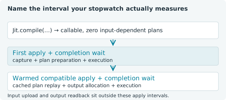
Choose Run all, then modify one experimental choice at a time. All compiled calls below run on CPU because this browser bridge rejects generated JIT kernels. A final optional GPU cell measures eager operations instead. Each lesson owns an independent Java session; leaving or reloading discards edits and cached plans. Measurements vary with the machine and concurrent activity.

1. Separate callable construction from first application

Jit.compile returns a callable before it has seen an input shape. Timing that constructor alone does not time input-dependent capture or compilation. The first application will do more work. We print the initial cache count to make that distinction observable without guessing from elapsed time.

The input contains 4,096 values cycling through 0, 1, 2, 3. This fixture is deterministic and modest enough for the emulated JVM. We keep it as a Java array between cells and create owned tensor inputs inside each experiment.

Expect zero plans. System.nanoTime() is useful for elapsed intervals; its absolute value is not a wall-clock timestamp. Convert a difference to milliseconds by dividing by 1e6. Timer precision does not remove noise from VM scheduling, browser activity, resource management or the operating system.

2. Measure a synchronized first application

Input creation and its completion happen before the timer starts. Inside the timing window, we apply the callable and wait for the output backend to finish. The timer stops before printing and output cleanup. This defines a specific boundary that you can describe to another reader.

If you rerun this cell with the same compiled object, it is no longer a first-call measurement. Rerun setup to obtain a fresh empty cache first. Even then, the process and underlying runtime may already be warm.

Expect one plan and the first four outputs [3, 4, 7, 12]. The interval includes capture, plan preparation, any backend compilation reached by this call, and execution through completion. It is not an isolated compiler timer. Subtracting a later replay time does not magically isolate compilation either: both intervals can differ in allocation, initialization and scheduling.

The output array is retrieved only after the elapsed value has been recorded. Readback still happens; it simply belongs outside this particular interval. A useful report names that exclusion rather than leaving readers to infer it.

3. Collect warmed replay samples

Warmup gives compatible calls a chance to reuse the plan and initialize recurring runtime paths. It does not establish a universal steady state after an arbitrary number of iterations. For this teaching example, three warmups and seven samples keep the experiment small and the code readable.

Every sample starts after input completion, includes output completion, and stops before output cleanup. Replay still includes the output allocation performed by apply; we have not built an allocation-free benchmark.

Change the sample count from seven to eleven, rerun, and look for variability. More samples help reveal a distribution; they do not repair an interval that measures the wrong boundary. Avoid printing inside the timed region or mixing unrelated work onto the same backend while collecting samples.

4. Report the sample distribution and cache state

A median is the middle sorted observation. It is less sensitive to one large outlier than the arithmetic mean, but it still describes only these samples. We also print the minimum, maximum, input length and current plan count so a single number does not conceal all the experimental conditions.

The supplied sample count is odd, so the middle element is the median. If you choose an even count, average its two middle elements instead. These statistics describe the measured synchronized Java-call intervals. They do not separate kernel duration from guest interpreter overhead or backend bookkeeping.

Try this: change the input length to 8192 in setup, then rerun all cells. That setup also creates a fresh callable, so you have a new cold experiment. If you retain the existing callable and apply a different shape instead, its cache may gain another plan. Chapter 3 explains those signature boundaries.

5. Give host readback its own interval

This CPU example first completes the output, then times only toFloatArray(). The method creates a Java array and obtains its values from the backend. On CPU this is a host-side download or copy path, not a PCIe transfer. On GPU it also involves retrieving device data through that backend's readback path.

The timer excludes the tensor calculation, but includes whatever allocation and conversion toFloatArray() performs. Checking the values after the timer keeps reporting separate while ensuring we have an understandable numerical fixture.

With the original 4,096-element fixture the checksum is 26624: each block of four contributes 3 + 4 + 7 + 12 = 26, and there are 1,024 blocks. This is a derived reference, not a recorded run. If you double the length while preserving the pattern, the checksum doubles too.

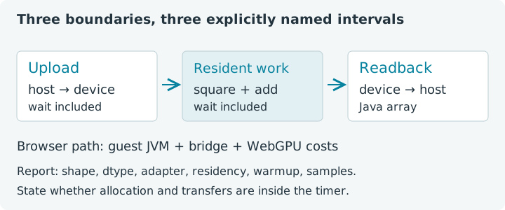
6. Separate the browser GPU's three boundaries

The final cell intentionally initializes the adapter before timing. It then measures upload, resident eager operations through completion, and completed readback separately. The arithmetic is the same, but execution is not JIT replay: square and scalar addition are individual supported bridge operations. Do not present these intervals as a CPU-versus-GPU benchmark.

Backend synchronization can include other outstanding work. The browser path also includes command serialization, VM communication and JavaScript scheduling. A native wgpu application has a different path and needs its own measurements.

Expect the first four values [3, 4, 7, 12] when the GPU cell runs. These are single observations for learning the boundaries. Availability checks and adapter setup have already happened, but the first dispatch may still include pipeline initialization. Repeating the cell changes that condition; report whether a run was fresh or warmed.

For an application measurement, record the jax4j version, engine, adapter, shape, dtype, input residency, warmup, sample count and inclusion of allocation, synchronization and transfers. Use a controlled native Java harness for native performance claims. Keep a separate end-to-end measurement if your actual request also includes input preparation and result consumption.

Return to capture rules and cache keys when a shape change surprises your cache count, or to batching with vmap when repeated small calls suggest a better-shaped workload. A timing number becomes useful when you can say exactly what work it represents.