Matrix multiplication and linear algebra

Three features become two outputs

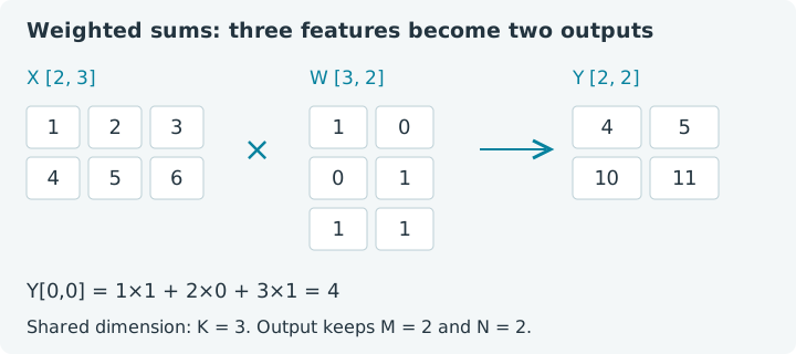
A batch contains two observations, each with three features. You want two weighted combinations of those features for every observation. This is the shape of a small linear layer, a pair of scoring rules, or a change of coordinates. Matrix multiplication expresses the weighted sums in one operation.

Our feature rows are [1, 2, 3] and [4, 5, 6]. The first output adds feature one to feature three; the second adds feature two to feature three. That gives [4, 5] and [10, 11]. We can check every entry before running anything.

Later in this notebook we will reverse a different calculation by solving a small linear system, then reconstruct a matrix from a triangular factor. These are constructed examples with simple reference answers, chosen to make the dimensions and numerical checks visible.

Choose Run all for the worked examples, then change individual cells. This page starts a separate Java session, loads the bundled jax4j 0.2.1 core, and uses CPU execution. Earlier lesson imports do not carry across pages. The browser JVM is emulated; its timings are not native performance results.

1. Match the shared dimension

For rank-two matrices, [M, K] × [K, N] produces [M, N]. The two occurrences of K must match. Each output entry sums K pairwise products. Here M = 2, K = 3 and N = 2: observations by features, multiplied by features by outputs.

Expect shape [2, 2] and flat output [4, 5, 10, 11]. The top-left entry is 1 × 1 + 2 × 0 + 3 × 1 = 4. The top-right uses the other weight column: 1 × 0 + 2 × 1 + 3 × 1 = 5. An output column chooses one set of feature weights; an output row retains one observation.

Try this: change the last row of the weight matrix from [1, 1] to [2, 2], rerun setup, and predict the result. You should get [7, 8, 16, 17]. Both output rules now give the third feature twice the influence. Restore the original weights for the next reference answer.

mul would ask for elementwise multiplication with broadcasting. It does not perform these weighted sums. Do not use the two method names interchangeably: a shape can tell you that an operation is invalid, but cannot tell you that you chose the operation your model intended.

2. Add one bias per output

After multiplication, each observation has two outputs. A bias vector of shape [2] aligns with that final output axis and applies to both observations. This is the same broadcasting rule as in the first notebook of this chapter.

With the original weights, expect [4.5, 4.5, 10.5, 10.5]. Change the bias to [0, 10]: only the second output of each observation should shift. Then add another observation to features, update its row count, and rerun. The weight matrix remains [3, 2]; a different batch size does not require different feature weights.

That last edit is worth doing deliberately. The factory checks that the flat array length matches its requested shape. Matrix multiplication then checks the shared dimensions. Those checks catch different mistakes at different boundaries, before you interpret the output numbers.

Restore the original feature and weight arrays before comparing the following reference outputs.

3. Transpose when the question changes

x.transpose().matmul(x) forms a feature-by-feature matrix: [3, 2] × [2, 3] produces [3, 3]. Each entry is a dot product between feature columns across observations. This uncentered Gram matrix is useful for understanding the geometry of the data, but it is not automatically a covariance matrix.

The rows are [17, 22, 27], [22, 29, 36] and [27, 36, 45]. For example, the first diagonal entry is 1² + 4² = 17. The matrix is symmetric because the dot product between columns A and B equals the dot product between B and A.

Try x.matmul(xt) instead. You get a two-by-two matrix comparing observations, with rows [14, 32] and [32, 77]. The same values answer a different geometric question. A transpose changes both which dimensions align and which entities the output compares.

Now deliberately reverse the original product to w.matmul(x). It is valid for these dimensions and gives a three-by-three result, but it is not the original observation-to-output mapping. “The multiplication worked” is only the beginning of the correctness check.

4. Solve for an unknown vector

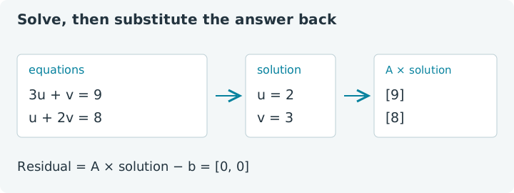
Suppose two unknowns satisfy 3u + v = 9 and u + 2v = 8. In matrix form, this is A × solution = b. The answer is u = 2, v = 3. solve expresses that question directly without requiring you to construct an inverse matrix.

The solution is [2, 3], and this example's maximum absolute residual is zero. A residual is the discrepancy left after substituting your answer back into the original equation. It is a much more informative check than simply printing the solver's output and hoping it looks plausible.

Change b to [5, 5] and predict [1, 2]. Check the residual again. Then use non-integer inputs: a tiny nonzero residual is normal in floating-point arithmetic. In general, interpret it relative to the scale of your inputs; a small residual alone does not guarantee an accurate solution when the system is poorly conditioned, meaning small input changes can strongly affect the answer.

In jax4j 0.2.1, solve and these dense factorization routines download to the host, perform their calculation there, and upload results to the original device. They are not native GPU factorization kernels. This notebook explicitly uses CPU, where that distinction is straightforward. The ordinary tensor matmul operation is dispatched through its selected backend.

5. Rebuild a matrix from a factor

For a symmetric positive-definite matrix, Cholesky factorization finds a lower triangular matrix L such that A = L × Lᵀ. Positive definite means every nonzero vector has a positive quadratic form vᵀAv. Our example [[4, 2], [2, 5]] has the particularly friendly factor [[2, 0], [1, 2]].

Expect [2, 0, 1, 2] for the factor and [4, 2, 2, 5] for the reconstruction. Multiply the small matrices by hand to verify each entry. As a coding exercise, add a residual calculation like the solver cell's rather than relying only on the printed arrays.

Try replacing the final diagonal entry 5 with 3. The matrix remains positive definite, but the last factor entry becomes approximately √2. Your reconstruction can now have a small rounding difference. Keep it separate from a genuinely invalid factorization, such as a matrix that is not positive definite.

6. Catch a dimension mismatch

The original feature matrix has three columns. A weight matrix with two rows cannot consume it. This deliberate failure is caught so the rest of the notebook remains runnable.

For a final experiment, choose one output instead of two. Make the weights [1, 0, 1] with shape [3, 1]. Predict shape [2, 1] and values [4, 10]. Then change the weights so the output is the average of the three features. You have built two different linear maps without changing the observations.

Every temporary in these examples has an explicit owner in a try resource list. That includes transposes, residuals and factor tensors. If you explore factorizations returning several tensors, inspect their result object and close each owned tensor; a Java record holding results is not automatically a resource scope.

You can now distinguish elementwise arithmetic, axis reductions and matrix products by the question each answers. Revisit broadcasting to add a per-output bias, or reshape, slice and reduce to select one run before a linear transformation. Continue with differentiating a scalar loss to use these building blocks in Chapter 2.