Forward and reverse mode: JVPs and VJPs

Two inputs, three outputs, one question at a time

Suppose f(u, v) = [u², uv, 3v]. At [2, 3], the outputs are [4, 6, 9]. If we increase u and decrease v by the same small amount, which outputs change fastest? Alternatively, if the outputs have weights [2, 1, -1], how sensitive is their weighted total to each input?

These questions use the same local derivative information in opposite directions. A Jacobian is the array of all output derivatives with respect to all inputs. We can multiply by it without building the entire array. A JVP pushes an input direction forward; a VJP pulls output weights back. Their names stand for Jacobian-vector product and vector-Jacobian product.

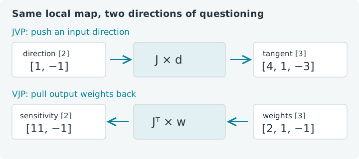
Choose Run all, then alter directions and weights in the individual cells. This notebook uses the bundled jax4j 0.2.1 CPU backend in the browser's emulated JVM. The small outputs are reference calculations, not performance measurements. Reloading discards your edits and session; each lesson starts with fresh imports.

1. Keep the function in tensor space

The function below selects two scalar slices, forms three expressions and stacks them into a vector. Selecting a scalar from shape [2] removes its leading axis, and stacking the three scalars creates shape [3]. These are the slicing and stacking operations from Chapter 1, now participating in a derivative calculation.

Inside these transforms, temporary traced tensors belong to the transform's scope. We close the ordinary input tensors and each tensor returned by the result records. The records themselves do not implement automatic cleanup.

2. Push one direction forward

A tangent is an input perturbation direction, not another set of input values. For direction [1, -1], imagine evaluating the function at [2 + epsilon, 3 - epsilon]. The JVP gives the first-order output change per unit of epsilon, evaluated at the original point.

Expect value [4, 6, 9] and tangent [4, 1, -3]. The three derivatives are 2u × du = 4, v × du + u × dv = 3 - 2 = 1, and 3 × dv = -3. The tangent follows the output shape, [3], because it describes output changes.

Try this: change the direction to [1, 0]. Expect [4, 3, 0], which isolates sensitivity to u. Then try [0, 1], giving [0, 2, 3]. These are the two columns of the Jacobian. Changing the point instead changes the local linear map itself: at [1, 3], the derivative of u² with respect to u is 2, not 4.

A tangent predicts small changes locally. For the original direction, the first output at [2 + epsilon, 3 - epsilon] is 4 + 4 epsilon + epsilon². The JVP supplies the coefficient 4; it does not include the quadratic remainder. Try epsilon = 0.1 on paper to see exactly where a finite move departs from its linear prediction.

3. Pull one set of output weights backward

A cotangent supplies weights for output sensitivities. Here [2, 1, -1] defines the scalar combination 2 f₀ + f₁ - f₂. Its derivative with respect to [u, v] is [4u + v, u - 3], giving [11, -1] at our point. The VJP computes that result directly.

jax4j's vjp accepts a function, inputs and explicit output cotangents in one call. It returns the original output and the resulting input cotangents; this API does not return a reusable pullback function.

Try weights [0, 1, 0]. Only the middle output contributes, giving [3, 2]. Next try [1, 0, 0]: the result is [4, 0]. You are selecting or combining output questions; the input point remains fixed. Multiplying all weights by two doubles the sensitivities without changing the original output.

If you picture gradients as column vectors, the returned cotangent is Jᵀw. The term “vector-Jacobian product” uses the equivalent row-vector expression wᵀJ. The API returns a tensor shaped like the input, [2]. Picking a consistent orientation on paper prevents a surprising amount of confusion.

4. Recover a familiar scalar gradient

Weights of all ones ask about the sum of all outputs. We can compare the VJP question with a scalar objective: grad(t -> function.apply(t).sum(), x). The next cell uses that scalar form and should give [7, 5].

Return to the VJP cell, replace the weights with [1, 1, 1], and check that it produces the same answer. Then use [1, 1, 0] and predict [7, 2]. The scalar loss from the previous lesson fits this pattern: a reverse pass starts with weight one on its single output, then accumulates contributions back to every input.

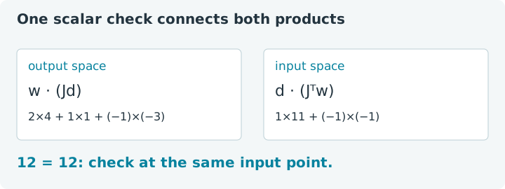
Here is a compact consistency check to try with ordinary arithmetic: [2, 1, -1] · [4, 1, -3] = 12, and [1, -1] · [11, -1] = 12. This identity relates a forward product and a reverse product of the same local map. It is useful when checking derivative implementations because it checks their agreement without requiring the full Jacobian. It does not establish correctness if both implementations share a matching mistake; hand calculations still earn their place.

5. Zero direction means zero first-order change

Forward differentiation is linear in the tangent. A zero tangent must produce a zero output tangent, although the function value remains unchanged. This is a useful way to separate the point where the function is evaluated from the direction you are asking about.

Expect [4, 6, 9] followed by [0, 0, 0]. Now change fullLike(0) to fullLike(2). The direction becomes [2, 2], and the tangent is [8, 10, 6]. It is twice the sum of the two basis-direction results from the earlier experiment. This linearity is in the direction at a fixed point; our original function remains nonlinear in its inputs.

6. Shapes describe different spaces

The JVP input tangent must match the input's shape, dtype, backend and device. The VJP output seed must match the output's shape, dtype and device, and its structure for structured outputs. In our example, confusing a two-element input direction with a three-element output weight vector is an error. The next cell deliberately supplies the wrong tangent shape.

Keep this cell as a failure example. Use the earlier successful JVP cell when experimenting with a valid two-element tangent: its try block closes both returned tensors. Changing this cell to succeed without adding cleanup would leave those handles unmanaged.

Forward mode is useful when you have a small number of input directions to explore; reverse mode is useful when you have a small number of scalar output combinations. Building a full Jacobian changes the cost question: one can sweep input basis directions or output basis weights. Neither mode is universally faster, and these examples do not claim a benchmark.

Continue with Jacobians, Hessians and nested derivatives to materialize the whole local map and then ask about curvature. The scalar-loss notebook is a useful reference when deciding what your output weights should mean.