A small network with explicit parameters

A network small enough to calculate on paper

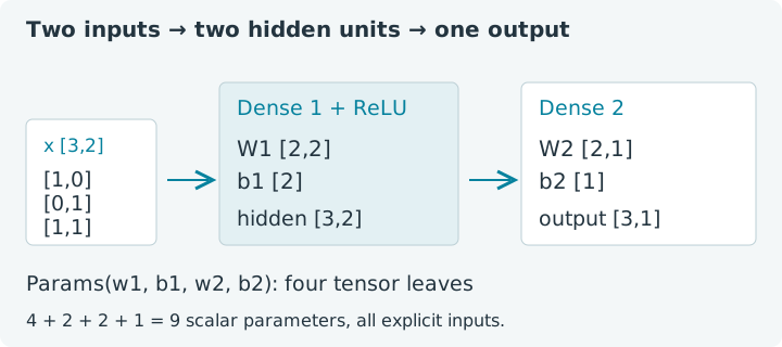
Three observations are [1, 0], [0, 1] and [1, 1]. Our network will initially predict [1.5, 1.5, 3]. The first two predictions are equal even though the observations use different features. We can explain that result by inspecting two small weight matrices, rather than trusting an opaque model.

The network has two inputs, two hidden units and one output. Its calculation is hidden = relu(x W1 + b1), followed by prediction = hidden W2 + b2. A dense layer applies a shared matrix and bias to each observation. ReLU sets negative entries to zero, creating a piecewise nonlinear function.

Choose Run all, then change weights, biases and observations. This notebook uses jax4j 0.2.1 on the emulated CPU. Each lesson starts its own Java session; typed declarations and helper methods persist between its cells. Leaving or reloading discards those declarations and your edits. These are constructed examples for understanding a model, not performance measurements.

1. Put parameters in a readable record

Params has four tensor leaves. The record organizes them; it does not create them, mutate them or close them automatically. predict receives both that record and the feature tensor explicitly. There is no hidden mutable parameter store inside the prediction function.

Dense.forward handles the matrix product and bias. The helper closes its preactivation and hidden tensors while returning the independently computed output. That makes the same function usable for ordinary inference and inside transforms, whose tracing contexts manage their own temporary allocations.

The shapes establish the architecture. w1 maps two features to two hidden units; w2 maps those two hidden values to one output. Biases have shapes [2] and [1], aligning with their layers' final dimensions. The batch length can change without changing either weight matrix.

Keep the helper as a pure calculation. Printing belongs after it returns; reading a traced value into Java would conflict with compilation or differentiation. The helper's parameters are ordinary explicit arguments, so later notebooks can ask for derivatives with respect to their leaves.

2. Choose recognizable initial values

We initialize W1 with rows [1, 0.5] and [0.5, 1], both hidden biases to zero, both output weights to one and the output bias to zero. These values are chosen for an inspectable example. Random initialization becomes useful for larger networks, with key handling following Chapter 4.

A factory returns a fresh owned parameter tree for each experiment. Closing one experiment's parameters therefore does not invalidate another cell's copy.

The tree contains nine scalar parameters: four in w1, two in b1, two in w2 and one in b2. Nine values are enough to see the relationships between architecture, shape and ownership without scrolling through a parameter listing that looks like a small telephone directory.

Try this: change the output bias from 0 to 1 in the factory. Every prediction in the next cell should increase by exactly one. Rerun this factory cell before rerunning inference, then restore the original value for the following reference answers.

3. Run three observations together

The feature matrix has shape [3, 2], with one observation per row. The prediction keeps that observation dimension and ends with one output channel, so its shape is [3, 1]. Printing a flat Java array does not remove that last singleton dimension.

Expect shape [3, 1], predictions [1.5, 1.5, 3] and four parameter leaves. For the first observation, the first dense layer produces [1, 0.5]. ReLU leaves both entries unchanged, and the output layer sums them. The second observation produces [0.5, 1], which has the same sum.

Change the output weights to [2, 1] in the factory. The predictions become [2.5, 2, 4.5]: the first hidden unit now contributes twice as much. Changing a named parameter leaf lets you predict which part of the computation will respond. Restore [1, 1] before continuing.

4. Inspect the hidden representation

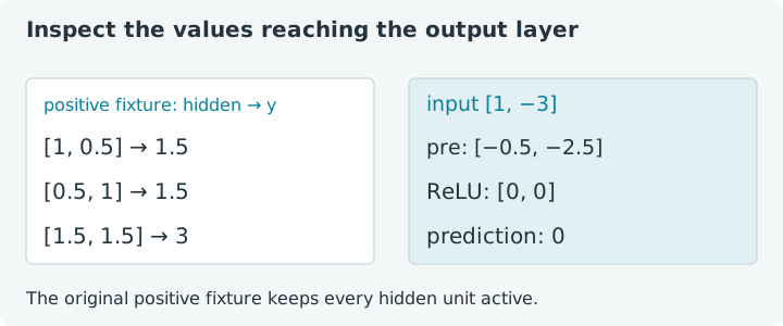
A hidden layer is just another tensor calculation. We can print the values before and after ReLU to understand what information reaches the output. On this positive fixture, all six preactivations are positive, so the nonlinearity currently leaves them unchanged.

Both arrays are [1, 0.5, 0.5, 1, 1.5, 1.5], representing three rows of two hidden values. Try adding a negative hidden bias and work out which units turn off first. A shared bias changes that unit for every observation; it does not belong to one particular row.

5. Make the activation change the answer

Use observations [1, -3], [-3, 1] and [1, 1]. The first two have negative preactivations in both hidden units. ReLU suppresses those values; the last observation remains active. This reveals behavior that the original positive-only fixture could not show.

Expect [0, 0, 3]. Replacing ReLU with an identity operation would give [-3, -3, 3], so the activation has changed the function materially. To try that edit with explicit ownership, replace pre.relu() with pre.mul(1), which creates a new identity-valued tensor rather than borrowing pre.

ReLU also affects gradients. In this implementation, negative entries have zero local derivative, and zero itself uses the implementation's chosen zero rule. The next lesson uses strictly positive hidden preactivations to keep its hand-calculated gradients away from that nonsmooth boundary.

6. Compile explicit parameters and features together

A compiled tree can contain both the parameter record and the input batch. ForwardInput names those two parts. Changing their runtime values with the same tree structure and leaf signatures can reuse a captured plan.

Expect [1.5, 1.5, 3], [0, 0, 3] and one plan. The parameters are runtime tensor leaves, not a Java closure hiding fixed weights. Adding a fourth observation changes the feature shape and creates another specialization, while the layer weight shapes remain unchanged.

Continue with a loss function and its parameter gradients to compare these predictions with targets. Revisit parameter trees for cache structure and the distinction between a container and its tensor owners.