A compiled training step with functional Adam

The optimizer has state too

A training step needs more than a parameter gradient. Adam carries a moving average of gradients, a moving average of squared gradients and a step count used for bias correction. If those quantities are hidden Java mutations inside a captured function, replay does not describe the complete update.

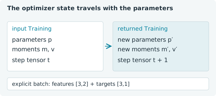
FunctionalAdam exposes that state as tensor trees. Our compiled step will receive the network parameters, optimizer state, features and targets, then return fresh parameters and fresh optimizer state. The feature batch remains owned by its caller. The first loss is still 13 / 6 for the small network from the previous two lessons.

Choose Run all, then adjust the learning rate or iteration count. This standalone notebook uses jax4j 0.2.1 on the emulated CPU. Its tiny constructed fixture teaches state and ownership; it is not a training-speed or generalization benchmark. Reloading discards edited code, parameters, optimizer state and caches.

1. Keep the same network

The two-layer forward function still receives all four parameter tensors explicitly. It owns ordinary temporary activations and returns a new prediction tensor. We repeat its definition so this notebook does not depend on another page's Java session.

2. Reuse the parameter factory and scalar loss

The initial weights give predictions [1.5, 1.5, 3] for feature rows [1, 0], [0, 1] and [1, 1]. We keep targets [2, 3, 5] shaped [3, 1]. Those shapes pair each prediction with its own target, avoiding the accidental all-pairs broadcast from the previous lesson.

The loss remains a mean of squared residuals. Adam changes the update rule; it does not choose the objective or repair an incorrect target layout.

The parameter tree contains nine scalar values across four leaves. Adam's first- and second-moment trees mirror those same shapes. Its step is a separate one-element F32 tensor, so replay can use the current count without a host read.

For reference, all nine initial parameter derivatives are negative in this fixture. With zero moments, Adam's bias-corrected first update is approximately one learning-rate unit in the positive direction for every parameter. The small epsilon in the denominator and F32 arithmetic make that an approximation.

3. Capture the complete training step

Training contains parameters and optimizer state. StepInput adds the batch features and targets. The body computes parameter gradients, calls the functional optimizer, closes the temporary gradient tree and returns the next state. No application code reads the step tensor during capture.

FunctionalAdam.update is itself implemented with a compiled pure update; this outer composition follows the same explicit state contract. The learning rate, beta coefficients and epsilon are Java configuration belonging to the optimizer object. Changing that configuration means creating the appropriate optimizer and compiled callable, rather than assuming a tensor-state update changes those constants.

The defaults are beta1 = 0.9, beta2 = 0.999 and epsilon = 1e-8. At each step, Adam forms moving averages of the gradient and its square, bias-corrects them using the incremented count, and scales the parameter update by the corrected second moment's square root plus epsilon.

4. Initialize moments and inspect the state

Initialization creates zero first moments, zero second moments and step zero. The helper below gives every experiment a fresh parameter tree and matching optimizer state. The returned record owns those tensors as a group in these examples, so whole-tree cleanup is appropriate.

Expect step 0 and two zero entries for each displayed moment. These are tensors with the same shapes as w2, not a Java counter and a pair of host-side arrays. All other parameter leaves have corresponding moment leaves.

Reinitializing moments on every iteration would ask a different optimization question. The following cells initialize once per experiment and feed each returned state into its next update. A Java loop controls how many complete training calls to make; it does not mutate Adam's internals during capture.

5. Advance one step and inspect the new loss

The new state has step one. For this fixture, the first update should move the output bias from zero to about 0.01. The independently derived idealized predictions are approximately [1.5654, 1.5654, 3.1006], giving loss about 1.95156. These references ignore tiny epsilon and F32 bias-correction effects.

Expect step 1, output bias near 0.01, loss near 1.95156 and one outer training plan. The reported loss is evaluated after the update; the gradients used to produce that update came from the previous parameters. Keeping those two times distinct matters when comparing a training log with a hand calculation.

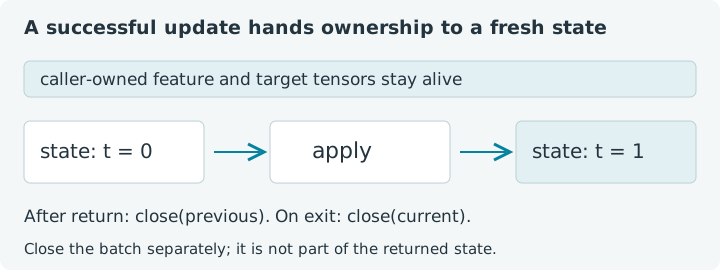
The assignment happens before closing the previous state. If train.apply fails, the current state remains available for the enclosing cleanup. After a successful return, the new parameter and moment leaves are independently owned, so releasing the old state does not invalidate them. This particular training function returns fresh state, not aliases of the input batch.

6. Replay with the latest state each time

The parameter values, moments and counter change while their structure and shapes stay fixed. Compatible calls can therefore reuse one outer training plan. The next experiment starts fresh, then performs ten updates on the same three-observation batch.

The step should be 10 and the outer plan count should remain 1 in the original sequence. Inspect the actual predictions and loss rather than assuming a particular convergence curve. Adam does not guarantee that every individual step reduces every objective. Try another rate by recreating the optimizer and training callable, then compare experiments from fresh initial state.

For a changing batch with the same feature and target shapes, supply its new tensor values explicitly. A new batch shape creates another specialization. Every replay must receive the latest returned optimizer state; repeatedly feeding the original state would repeatedly ask for a first step.

The three observations are the entire constructed training fixture, with no held-out set. Matching their targets establishes fit to this example, not a claim about unseen data. Revisit the parameter gradients when an update surprises you, and capture rules when new runtime values appear to be ignored.