A loss function and its parameter gradients

Which weights should change to fix three predictions?

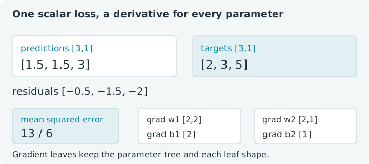
Our two-layer network predicts [1.5, 1.5, 3] for observations [1, 0], [0, 1] and [1, 1]. The targets are [2, 3, 5], chosen from the simple rule target = 2 × first feature + 3 × second feature. Every prediction is too low, but each parameter influences those errors differently.

The mean squared error is (0.5² + 1.5² + 2²) / 3 = 13 / 6, about 2.166667. We will differentiate that scalar with respect to the parameter record. The resulting gradient has the same four-leaf structure as the parameters, with each derivative tensor matching its parameter's shape.

Choose Run all, then modify a target or parameter and predict its effect. This notebook repeats the model helpers so it works in its own Java session. It uses jax4j 0.2.1 on the emulated CPU. Reloading discards declarations and edits. This is a constructed training fixture, not evidence of predictive accuracy on held-out observations.

1. Keep the model’s parameter input explicit

The architecture is unchanged: two dense layers with a ReLU between them. Params organizes the tensor leaves, and predict owns its temporary preactivation and hidden tensors. The returned prediction belongs to its caller. Inside differentiation, the tracing context keeps the values needed by its rules.

Differentiating the parameters is a different question from differentiating the feature inputs in Chapter 4. Here the observations and targets are fixed for one loss evaluation. The parameter tree is the argument whose sensitivities we ask the transform to return.

2. Define one scalar objective

The loss function subtracts targets from predictions, squares the residuals and averages all entries. Both predictions and targets must have shape [3, 1] for this fixture. Naming and closing the intermediate tensors also makes the helper safe to use for ordinary, untraced reporting.

The factory creates fresh tensors with the same hand-picked values as the previous notebook. Its original hidden activations are all strictly positive, so ReLU behaves locally as the identity for the derivative calculation below. That makes every gradient independently calculable with matrix products.

A mean reduction includes the factor 1 / 3. Replacing it with a sum multiplies every parameter gradient by three. Keep that scaling in mind when interpreting a learning rate or comparing the following reference fractions.

3. Inspect the output layer’s gradients

valueAndGradTree returns the loss plus a gradient tree. The lambda takes only the parameter record as its differentiated input; it uses the supplied feature and target tensors for this evaluation. Closing the returned record's tensor leaves does not close those inputs.

Expect loss about 2.166667, output-weight gradients [-17/6, -19/6] and output-bias gradient [-8/3]. The derivatives with respect to predictions are 2 × residual / 3 = [-1/3, -1, -4/3].

The bias contributes equally to every prediction, so its gradient is the sum of those three derivatives. Each output weight instead receives that derivative multiplied by its hidden activation. For example, the first weight gets 1 × (-1/3) + 0.5 × (-1) + 1.5 × (-4/3) = -17/6.

Try this: increase only the last target from 5 to 6. Its prediction derivative decreases by 2/3. The output-bias gradient decreases by 2/3, and each output-weight gradient decreases by 1 because that row's hidden activations are both 1.5. Restore target 5 for the next references.

4. Follow the error into the hidden layer

The hidden weights also receive gradients through the output layer. With both output weights initially one and all hidden preactivations positive, each hidden unit receives the same per-observation upstream derivative. Multiplying by the feature columns then gives the hidden weight matrix's gradients.

Expect w1 rows [-5/3, -5/3] and [-7/3, -7/3], with b1 equal to [-8/3, -8/3]. The first feature appears in observations zero and two, so its weight contributions sum to -1/3 - 4/3 = -5/3. The second feature appears in observations one and two, giving -1 - 4/3 = -7/3.

Change the second output weight from 1 to 2 in the factory and recompute. The predictions and residuals change too, so do not simply double the old hidden gradients. Chain-rule reasoning has to use the current forward values. Print the predictions before drawing conclusions from a changed gradient.

5. Apply one update to every parameter leaf

A gradient points toward increasing loss locally. The update p - 0.01 × g moves in the opposite direction. We use a small compiled tree to apply this same operation to corresponding parameter and gradient leaves; the tracing scope manages the expression's temporary scaled gradients.

The independent real-arithmetic reference is approximately 1.639449, below the initial 2.166667; F32 calculations can differ slightly. The corresponding predictions are about [1.6601, 1.6755, 3.254]. This is a derived reference for this specific update, not a recorded training benchmark.

Try another small rate and inspect both the predictions and loss. A larger step is not guaranteed to improve the objective. The updated tree contains new tensors, so we close it separately from the original parameters and gradients. A record is a structure, not an in-place parameter update mechanism.

6. Check target shape before trusting a loss

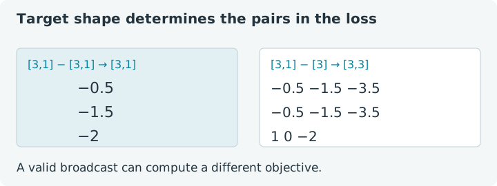
A target vector of shape [3] is not interchangeable with targets of shape [3, 1]. Subtracting it from predictions of shape [3, 1] broadcasts to [3, 3], comparing every prediction with every target. That operation succeeds while asking the wrong training question.

Expect [3, 3] and [3, 1]. Inspect a few entries in each residual tensor. The correct objective pairs observation zero with target zero, rather than letting a convenient broadcast define the pairing for you.

Continue with a compiled training step with functional Adam to carry optimizer state explicitly across updates. Revisit broadcasting whenever a loss looks plausible but its tensor shapes tell another story.