Custom JVPs, VJPs and checkpoints

A derivative rule is part of the operation’s contract

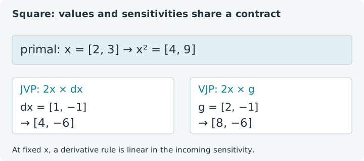
The function is square(x) = x². At [2, 3], its values are [4, 9]. An input tangent [1, -1] should produce output tangent [4, -6]. Output weights [2, -1] should pull back to [8, -6]. These small numbers let us check a custom rule before trusting it inside a larger model.

CustomDerivative wraps a pure tensor function with an explicit JVP or VJP rule. The forward function still defines the values; the rule defines how a transformation propagates sensitivities. A wrong rule can give plausible values and incorrect derivatives, so the agreement between them is your responsibility.

Choose Run all, then change a function and its rule together. This notebook uses jax4j 0.2.1 on the emulated CPU. Typed custom operations persist between cells. Ordinary input and result tensors have explicit owners; traced rule intermediates belong to the enclosing transform's scope. Reloading discards edits and Java state.

1. Specify the primal and a tangent rule

A custom JVP receives the primal input x and incoming tangent dx, and returns the output tangent. For a square, that is 2 × x × dx. The rule must be linear in the tangent at a fixed input. Returning the squared tangent, for example, would not describe the derivative of this function.

The derivative tensor must match the forward output's shape, dtype and placement. Keep the callbacks in tensor operations so the transform can inspect and compose their calculation. Host reads inside differentiation remain unsupported.

This square does not need a custom derivative in normal use: jax4j already knows how to differentiate multiplication. We deliberately use a familiar operation to make the contract transparent. Specialized implementations can need a rule with a more suitable numerical formulation, but the same correctness obligation applies.

Try this on paper first: replace the primal with a cube. The matching JVP is 3 × x² × dx, not 2 × x × dx. At [2, 3] and direction [1, -1], its output tangent would be [12, -27]. Restore the square rule before comparing the following reference results.

2. Push the direction through the custom operation

Transforms.jvp returns both the forward values and the tangent produced by our custom rule. The returned record is a container; close each tensor it owns. Inspecting both values prevents a derivative-only check from overlooking an incorrect primal function.

Expect [4, 9] followed by [4, -6]. Double the direction and the tangent doubles while the values stay fixed. Replace the direction with zero and the tangent becomes zero. These are simple linearity checks for a JVP rule at a fixed primal input.

In this API, reverse differentiation can also be derived from a custom JVP by transposing its tangent-linear calculation. A rule that breaks that linearity undermines this route as well. Shape validation can catch incompatible tensors; it cannot establish that your mathematical derivative is correct.

3. Define a direct pullback instead

A custom VJP receives the primal input x and the incoming output cotangent g. It returns an input cotangent. For an elementwise square, the pullback is 2 × x × g. The multiplication looks like the JVP rule here because the local Jacobian is diagonal; a general vector-valued operation requires the correct transpose action.

Expect [4, 9] and [8, -6]. Set the weights to [1, 1] and predict [4, 6], matching the gradient of the summed square outputs. Then select only the second output with [0, 1], giving [0, 6].

A custom VJP can be useful when the reverse calculation has a convenient implementation. It does not automatically provide a forward-mode rule in this release. The next example makes that supported-mode boundary visible.

4. A VJP-only operation rejects a JVP

The forward values can be computed, but asking a VJP-only custom operation for an output tangent is unsupported. Catching this error documents the contract and lets the rest of Run all proceed.

Use the earlier custom JVP cell for successful forward-mode experiments; it closes both returned tensors. Keep this cell as a deliberate failure, or add equivalent cleanup if you change it to a supported operation. Choosing a rule API should account for the transforms your callers need, including higher-order compositions.

5. Recompute a pure block during the pullback

A checkpoint changes how a block's derivative is obtained: the reverse pass recomputes its pure forward calculation instead of retaining its internal differentiation tape. This trades saved internal intermediates for additional work. It preserves the intended function and derivative.

Our block is (x² + 1) × x, or x³ + x. At [2, 3], it produces [10, 30]; the summed value is 40 and its gradient is [13, 28]. Those exact polynomial references make the comparison easy to inspect.

Expect 40, [13, 28] and same gradient: true. Change the input to [1, 2]: the summed value becomes 12 and the gradient becomes [4, 13]. Then modify the block to x³ + 2x by replacing the internal add(1) with add(2). At the original input, predict value 45 and gradient [14, 29]. Recreate the checkpoint after changing the block.

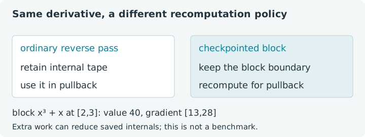
This tiny block is an illustration, not a memory or speed benchmark. A checkpoint does not remove the input, output or all working storage. Pick useful boundaries in a larger calculation and measure the actual tradeoff there. Recomputed code must represent the same function: mutable Java effects or newly chosen random inputs would change what is being differentiated. Pass deliberate tensor inputs and keep any key derivation reproducible.

6. Differentiate the rule at another order

The custom JVP rule is itself made of transformable tensor operations. For the summed square outputs, the Hessian should be the two-by-two diagonal matrix with entries 2. This is a compact second-order check of the rule's dependence on the primal input.

Expect shape [2, 2] and flat values [2, 0, 0, 2]. Try another input: the square's curvature stays constant. For a consistent cube primal and JVP, the Hessian at [2, 3] would instead have diagonal entries 12 and 18. Unsupported operations or missing derivative modes in a callback can still limit a composition; a custom rule does not bypass those requirements.

Return to JVPs and VJPs for their directional and weighted-output meanings, or Jacobians and Hessians when choosing which derivative representation to request. A custom primitive and a checkpoint both deserve the same careful numerical checks as the original function.