GARCH and maximum likelihood: a tape too big to JIT
The same adjoint machinery every calibration in this module used, pointed at a Gaussian log-likelihood over a return series instead of an option surface — until the series gets long enough to outgrow the fast engine.
Every calibration so far in this module has fit a model to option prices. GARCH(1,1) fits a model to a return series instead — there's no option, no strike, no payoff, just the Gaussian negative log-likelihood of how a variance evolves day to day. It's the same recorded-tape, adjoint-gradient machinery 7.1 opened this module with, pointed at a completely different kind of target. The twist is size: an option's tape has a few dozen nodes. A return series's tape has one recursion step per observation, and at realistic sample sizes, that's enough nodes to break the engine every other page in this module has defaulted to.
The whole story
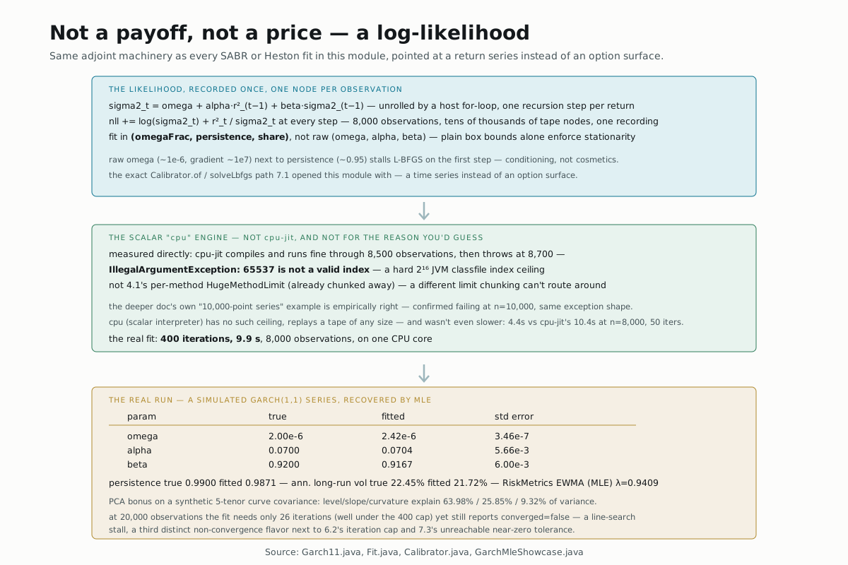
Garch11.fit doesn't optimize (omega, alpha, beta) directly — it fits
(omegaFrac, persistence, share) instead, where omega = omegaFrac × sampleVariance, persistence = alpha + beta, and share = alpha / persistence. The source comment is specific about why: raw omega
(~1e-6, with a gradient around ~1e7) sitting next to persistence
(~0.95) stalls L-BFGS on its very first step, because the two coordinates
live at wildly different scales. Reparameterizing also turns three coupled
inequality constraints (omega > 0, alpha, beta ≥ 0, alpha + beta < 1)
into three independent box bounds — the exact same Calibrator.of /
solveLbfgs path 7.1 used for SABR, unmodified, just handed a
differently-shaped problem.
One recursion, unrolled by a host loop
The whole model is one Java for loop building ADouble arithmetic, once
per observation, with no branch and no early exit:
ADouble s2 = rec.constant(var0);
ADouble nll = rec.constant(0.0);
for (double ret : returns) {
  ADouble r2 = rec.constant(ret * ret);
  nll = nll.add(s2.log()).add(r2.div(s2));
  s2 = omega.add(alpha.mul(r2)).add(beta.mul(s2));
}
rec.output(nll.mul(0.5));
Nothing here is different in kind from every other recorded objective in this module — it's still "build the arithmetic once, let the recorder do the rest." What's different is scale: 8,000 observations means 8,000 copies of that five-op body on one tape, tens of thousands of nodes for a series that's unremarkable by real risk-management standards (a year of daily returns is barely 250).
The engine choice, checked rather than trusted
The source comment for .on("cpu") says the tape is "past what the
straight-line bytecode kernel can emit." Rather than take that at face
value, I ran the same recording at increasing observation counts on both
engines. cpu-jit compiles and runs correctly all the way through 8,500
observations — and isn't even faster there: 50 identical iterations at
8,000 observations took 10.4s on cpu-jit against 4.4s on plain
cpu. At 8,700 observations, cpu-jit throws:
IllegalArgumentException: 65537 is not a valid index.
Entry: 10 com/nablatensor/engine/jit/JitKernel_Gen.rev$94-([D[D)V
65537 is 2¹⁶ + 1 — a hard JVM classfile index ceiling, not the
per-method 8,000-byte HugeMethodLimit 4.1 already covered. That earlier
limit is already handled: codegen chunks a large tape into many small
methods specifically to stay under it. This is a different, harder wall
those chunks can't route around — some shared per-kernel table is capped
at 65,536 entries no matter how the tape is split into methods. The deeper
doc's own illustrative number, "a 10,000-point series," turns out to be
accurate: 10,000 observations reproduces the same exception. cpu — the
scalar interpreter — has no such table and no such ceiling; it replays a
tape of any size, one node at a time, which is the entire reason this page
exists on the "safe" engine rather than the fast one.
Run the fit at 20,000 observations instead of the showcase's default
8,000 and the optimizer needs only 26 iterations — comfortably under
its own 400-iteration cap — yet still reports converged=false. Reading
Calibrator.solveLbfgs explains why: that's not the iteration cap 6.2's
BermudanLsm hit, or the unreachable-near-zero tolerance 7.3's Nelder-Mead
hit — it's the line search itself failing to find an accepted step within
30 backtracks (if (xNew == null) { break; }) and exiting early. A third,
structurally distinct way an optimizer in this codebase can stop without
certifying its own answer, on top of the two this Learn section had
already found.
The real run
An 8,000-observation return series simulated from (omega=2.0×10⁻⁶, alpha=0.07, beta=0.92) — persistence 0.99, a realistically slow-decaying
variance process — fit back by Garch11.fit:
| param | true | fitted | std error |
|---|---|---|---|
| omega | 2.00e-6 | 2.42e-6 | 3.46e-7 |
| alpha | 0.0700 | 0.0704 | 5.66e-3 |
| beta | 0.9200 | 0.9167 | 6.00e-3 |
Persistence recovers 0.9871 against a true 0.9900; annualized long-run
volatility 21.72% against a true 22.45%. Every fitted value sits within
roughly one to two of its own standard error of the truth — a real,
computed check, not just eyeballed closeness. 400 iterations (the hard
cap), 9.9 seconds, one CPU core. The same run also fits a RiskMetrics
EWMA decay by maximum likelihood (λ = 0.9409, close to the industry-
standard 0.94 this decay is famous for) and closes with a bonus PCA of a
synthetic 5-tenor curve covariance — level, slope, and curvature explaining
63.98%, 25.85%, and 9.32% of the variance, in that order, exactly the
shape a real yield-curve PCA produces.
Try it yourself
Run the showcase with -Dobs=20000 instead of the 8,000 default and
predict the iteration count and wall time before you run it. (26
iterations — far fewer, not more, because more data makes the likelihood
surface better-conditioned — but 11.6 seconds, still slower overall since
each iteration now costs 2.5× as much. Standard errors tighten across the
board too: beta's shrinks from 6.00×10⁻³ to 3.68×10⁻³.)
▶️ Run it
mvn -o -q -pl nablatensor-examples exec:java \
  -Dexec.mainClass=com.nablatensor.examples.GarchMleShowcase -Dobs=8000
No engine string to pass — Garch11.fit hardcodes cpu internally, for
the reason this page's second sidenote measures directly.
⚠️ What this doesn't do
Returns are assumed zero-mean, so this fits pure conditional-variance
dynamics with no separate mean equation — standard practice for short-
horizon returns, not a limitation this engine invented. Only plain
GARCH(1,1) is here, not the asymmetric (GJR, EGARCH) variants that let bad
news raise volatility more than good news does. And despite this whole
module being about adjoint gradients, the standard errors come from a
plain finite-difference Hessian (secondPartial, four nll() evaluations
per matrix entry) at the optimum, not a second adjoint sweep — the first
derivative is exact and cheap; the second one here quietly isn't.
What's next
→ Deeper: GARCH(1,1) maximum likelihood with an adjoint score
has the full estimate package table (Ewma, CorrelationEstimator,
Pca) and the pinned test tolerances this page's numbers are checked
against.
→ Module 7 (Calibration) is complete. Next: CDO tranches: two ways to price the same loss —
Module 8 opens with the first credit-risk topic in this Learn section.