Bootstrapping a curve: zero-rate risk for free
A rates desk hedges by instrument PV01, but a risk system reports by zero-rate bucket. Recording the bootstrap recursion once turns the map between them into one adjoint sweep instead of a curve re-solved per quote.
Every calibration so far in this module has fit a model's own parameters.
Bootstrapping a curve is a different problem wearing similar clothes: there
is no model, just a stack of swap quotes that a discount curve and one or
more forecast curves have to reprice exactly. A rates desk hedges each swap
by its own PV01, but a risk system reports exposure by zero-rate bucket
instead — someone has to compute the map between the two, d(zero rate) / d(quote), for every pillar against every quote. Re-bootstrapping the whole
stack once per quote just to bump it would work, but it's the same
one-Greek-at-a-time cost 2.1 already showed is avoidable.
The whole story
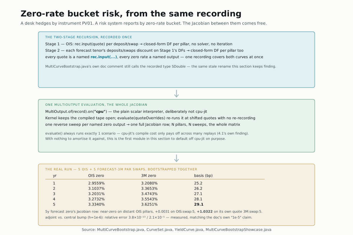
MultiCurveBootstrap's own doc comment states the point in one line: the
recorded recursion returns "the bucket-delta transformation a rates desk
applies to turn instrument PV01s into zero-rate risk." A PV01 says how much
one swap's value moves; a zero-rate bucket says how much one curve pillar
moves — they're related by exactly this Jacobian, and it comes from the same
recording that produced the curve, not a second calculation. (That same doc
comment calls the recorded type SDouble, not ADouble — the same stale
rename 7.1 traced through three other source files in this engine, now a
fourth.)
Two closed-form stages, no solver anywhere
MultiCurveBootstrap never iterates to find a discount factor. Because the
annual grid gives each swap exactly one new pillar, every stage's par-swap
equation solves in closed form for that one unknown:
// annual par swap: P(0,T) = (1 - q * prefix_{<T}) / (1 + q)
df = rec.constant(1.0).sub(q.mul(prefix)).div(rec.constant(1.0).add(q));
Stage 1 builds the OIS discount curve this way from OIS deposits and par
swaps. Stage 2 repeats the same closed-form move once per forecast tenor,
except the float leg and annuity of those swaps discount on Stage 1's own
oisDfByYear map — read directly in source, not assumed from the module's
name, this is where a forecast zero rate's dependence on OIS quotes actually
enters the tape, pillar by pillar, as the recursion runs. Every quote
becomes a named rec.input(inst.label(), inst.quote()), and every zero rate
becomes a named output (out.put("z:" + inst.label(), ...)) — one
recording, both curves, all ten quotes and ten zero rates on the same tape.
One Jacobian row per reverse sweep
MultiCurveBootstrap.Kernel wraps that recording in a MultiOutput and
keeps the compiled tape open, so the whole stack can be re-evaluated at
shifted quotes — a bump cross-check, a scenario — without re-recording:
this.mo = MultiOutput.of(rec -> record(rec)).on("cpu").build();
// ...
public Result evaluate(Map<String, Double> quoteOverrides) {
  MultiOutput.Result r = mo.run(quoteOverrides, 1L, 0L);
  // one r.gradient(zeroLabel) per zero rate -> one Jacobian row each
Each of the ten zero rates gets one reverse sweep, and each sweep's gradient is that zero rate's full row against all ten quotes — read back by name, the same mechanism 2.2 first traced. Because an OIS zero rate's recording never touches a forecast quote at all, its row is exactly zero there by construction, not by a later filter: the Jacobian is block lower-triangular because the tape itself only has edges running one way.
Look at that .on("cpu") and it's easy to assume a typo — every other
Monte-Carlo showcase in this section defaults to cpu-jit. It isn't one:
evaluate() always calls mo.run(quoteOverrides, 1L, 0L) — exactly one
scenario, every time, because there's nothing stochastic to replay. 4.1
already established that cpu-jit's bytecode-generation cost only pays for
itself across many replays of the same tape; with a scenario count of 1,
there's no "many" to amortize it against, so the plain scalar interpreter is
the faster choice here, not the default one. This is the first module in
this Learn section where cpu-jit genuinely isn't the right call.
The real run
MultiCurveBootstrapShowcase bootstraps five OIS par swaps against five 3M
forecast par swaps, 1y through 5y, at a real ~25bp starting tenor basis:
| yr | OIS zero | 3M zero | basis (bp) |
|---|---|---|---|
| 1 | 2.9559% | 3.2080% | 25.2 |
| 2 | 3.1037% | 3.3653% | 26.2 |
| 3 | 3.2031% | 3.4743% | 27.1 |
| 4 | 3.2732% | 3.5543% | 28.1 |
| 5 | 3.3340% | 3.6251% | 29.1 |
The basis widens from 25.2 to 29.1 bp across the curve — a real,
computed number, not an assumption from the ~25bp input quotes, since the
zero rate is a nonlinear transform of the bootstrapped discount factors. The
5y 3M forecast zero's Jacobian row is near zero against every OIS pillar
except the closest ones, +0.0031 against OIS:swap:5, and +1.0322
against its own quote 3M:swap:5 — a diagonal entry just over 1.0,
because a swap's own quote moves its own zero rate slightly more than
one-for-one once the annuity effect is included. Wrote and ran a standalone
probe (javac+java against the built classes, same approach as every
prior module) taking an independent central bump (h=1e-6) of that same
row: relative error 3.8×10⁻¹³ against the OIS entry, 2.1×10⁻⁶ against
the diagonal one — both comfortably inside the 1e-5 the deeper doc
claims, measured directly rather than taken on faith. Every one of the ten
calibrating instruments reprices to its own input quote to 8 decimal places.
Try it yourself
The showcase reprices a 4y receive-fixed swap struck at 3.30% (par 3.6100%, annuity 3.6963, PV -0.01146). Change the maturity from 4 to 5
and predict the new PV before you run it — both the par rate and the
annuity move. (par 3.6800%, annuity 4.5428, PV -0.01726: further
underwater, because the 5y par rate has risen further above the fixed
3.30% strike than the 4y par rate had.)
▶️ Run it
mvn -o -q -pl nablatensor-examples exec:java \
  -Dexec.mainClass=com.nablatensor.examples.MultiCurveBootstrapShowcase
No engine string to pass — MultiCurveBootstrap.Kernel hardcodes "cpu"
internally, for the reason this page's second sidenote traces.
⚠️ What this doesn't do
This is the stylised annual construction CurveSet's own doc comment names
directly: fixed and floating legs share one annual grid, so every swap adds
exactly one pillar and every stage solves in closed form. Real desks need
sub-annual float frequencies, interpolation inside the solve rather than
only on the finished curve, and cross-currency basis, none of which are
here. The deeper doc also flags that an analytic block Jacobian is a
possible faster alternative to the recorded-and-replayed one this page
walks through — YieldCurve.java's own doc comment even points at
CurveBootstrap (the single-curve version) as the place that already uses
one; MultiCurveBootstrap deliberately doesn't, favoring one general
mechanism over a bespoke analytic derivation per curve shape.
What's next
→ Deeper: Multi-curve (OIS) bootstrap with an adjoint Jacobian has the full builder API and the pinned test tolerances this page's numbers are checked against. → Next: Hull-White: swaptions from a root-find, not a tape — Module 7.5 prices a short-rate model whose own formula contains a solver, so it comes off the tape entirely rather than staying on it.