CDO tranches: two ways to price the same loss
A synthetic CDO tranche gets priced by two different models of the same one-factor Gaussian copula — a fast recursion with no gradient, and a recorded Monte-Carlo whose one adjoint sweep is the only way to get correlation delta.
A synthetic CDO slices a pool of credit names into tranches — equity absorbs the first losses, senior absorbs the last — and every tranche's value depends on the same thing: how correlated those names' defaults are with each other. Pricing a tranche's expected loss has a fast, exact recipe. But a trading desk doesn't just want the price — it wants to know how much that price moves if the market's view of correlation shifts, and the fast recipe has no gradient to give. So the same portfolio gets modeled twice.
The whole story
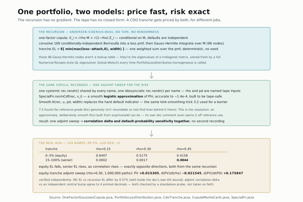
7.5 found that the reference-grade normal CDF genuinely can't be recorded —
HullWhiteCalibration's own doc comment named a root-find and N(x)
together as the two reasons that model stays off the tape. This module
resolves the second half of that: SpecialFn.normCdf's own doc comment
gives a smooth logistic approximation, 1/(1+e^{-(1.5976x+0.070566x^3)}),
accurate to about 1.4×10⁻⁴ — built entirely from exp/mul/add, so it
is tape-safe, and it's exactly what CopulaMonteCarlo uses to turn a
latent normal into a default probability inside a recorded tape. The same
doc comment is explicit about the trade: "for a reference-grade value use
com.nablatensor.quant.BlackScholes.N — that one is not tape-safe." Two
different normal CDFs, for two different jobs.
The recursion: fast, exact, no tape
OneFactorGaussianCopula starts from one identity: conditional on the
systemic factor M, every name's default becomes independent, with
probability Φ((Φ⁻¹(PD) − √ρ·M) / √(1−ρ)). PortfolioLossDistribution
convolves that conditional probability into a loss distribution one name at
a time — the Andersen-Sidenius-Basu recursion — then integrates over M
with Gauss-Hermite quadrature:
for (int g = 0; g < nodes; g++) {
  double m = Math.sqrt(2.0) * x[g];
  double p = OneFactorGaussianCopula.conditionalDefaultProbability(pd, rho, m);
  double[] cond = binomialPmf(names, p);
  // accumulate cond into the unconditional pmf, weighted by w[g]
}
CdoTranche.expectedLossFraction then reads a tranche's expected loss
straight off that distribution — one weighted sum over an integer default
grid, deterministic, no scenario count, no seed anywhere.
Those Gauss-Hermite nodes aren't a lookup table. gaussHermite builds the
three-term recurrence for Hermite polynomials into a symmetric tridiagonal
matrix and diagonalizes it with tqli — a full QL eigensolver with
implicit shifts, read almost line-for-line out of Numerical Recipes —
every single time PortfolioLossDistribution.homogeneous is called. The
96 quadrature nodes this page's numbers depend on are the eigenvalues of a
96×96 matrix, computed fresh, not cached and not hardcoded.
The same copula, recorded
CopulaMonteCarlo.trancheLoss builds the identical one-factor copula as a
tape instead: one shared systemic draw, one idiosyncratic draw per name,
and a smoothed comparison standing in for the hard default indicator —
ADouble xi = sqrtRho.mul(m).add(sqrtComp.mul(rec.randn()));
ADouble u = SpecialFn.normCdf(rec, xi);
defaults = defaults.add(Smooth.lt(rec, u, pd, width));
Smooth.lt is the same kink-smoothing move 3.2 used on a barrier option's
exercise boundary, here softening "did this name default" instead of "did
the spot cross the barrier." rho and pd are both named
Nabla.Inputs<CopulaMarket> reads, so .greeks() on the built pricer hands
back both a correlation delta and a default-probability sensitivity from
one reverse sweep — the recursion above can't give either, because nothing
about a Golub-Welsch eigendecomposition and a discrete convolution is
differentiable in the way an adjoint sweep needs.
The real run
CdoTrancheShowcase prices five tranches on a 100-name pool (PD=5%,
LGD=60%, 1y) at three correlations:
| tranche | ρ=0.15 | ρ=0.30 | ρ=0.45 |
|---|---|---|---|
| 0–3% (equity) | 0.6407 | 0.5175 | 0.4158 |
| 3–7% | 0.2019 | 0.2015 | 0.1864 |
| 7–10% | 0.0581 | 0.0931 | 0.1065 |
| 10–15% | 0.0159 | 0.0439 | 0.0633 |
| 15–100% (senior) | 0.0002 | 0.0017 | 0.0044 |
Equity falls and senior rises as correlation climbs — higher correlation
means defaults cluster, so the likely outcomes are "almost nobody defaults"
or "everybody does," which is bad for the tranche that only needs a few
defaults to be wiped out and good for the one that needs almost all of
them. The recorded copula Monte-Carlo on the equity tranche (ρ=0.30,
1,000,000 paths) gives protection-leg PV +0.015305, correlation delta
d(PV)/d(ρ) = −0.021545 (negative, as the table above already shows it
should be), and d(PV)/d(PD) = +0.175847. Wrote and ran a standalone probe
(javac+java against the built classes, same approach as every prior
module) to check both claims from the deeper doc directly rather than
trust them: the Monte-Carlo expected loss differs from the recursion's by
0.57% (the doc's own pinned test allows 6%), and the adjoint
correlation delta matches an independent central bump (h=1×10⁻³) to four
printed decimals (the doc allows 5%) — both comfortably inside their
claimed bounds, measured rather than assumed.
Try it yourself
Drop the pool from 100 names to 20 and rerun the correlation table.
Predict whether the equity-down/senior-up pattern still holds before you
check. (It does — equity falls 0.5347 → 0.4452 → 0.3650 and senior rises
0.0006 → 0.0025 → 0.0052 across the same three correlations, the same
direction as the 100-name table, just with a coarser loss grid: LGD ÷ names = 0.6 ÷ 20 = 0.0300, so one single name defaulting already uses up
the entire 0–3% equity tranche, landing exactly on its detachment point
rather than partway through it.)
▶️ Run it
mvn -o -q -pl nablatensor-examples exec:java \
  -Dexec.mainClass=com.nablatensor.examples.CdoTrancheShowcase
The recursion runs on the host, no engine string at all; the recorded
Monte-Carlo defaults to cpu-jit, the tranche's tape being small enough
(one shared systemic node plus a handful of ops per name) that nothing
here approaches 7.6's classfile ceiling.
⚠️ What this doesn't do
PortfolioLossDistribution.homogeneous assumes every name has the same
notional and the same loss given default — real portfolios don't, and the
class doc calls the heterogeneous case "a bucketed extension of the same
recursion" that this build doesn't implement. The copula itself is
one-factor: every name reacts to the same systemic shock, which is a
simplification real desks refine with sector or regional factors. And this
page never touches base-correlation bootstrapping from quoted index
tranches — the doc's own "Deferred" section names it directly as future
work, not a gap hidden by omission.
What's next
→ Deeper: Synthetic CDO tranches and correlation delta
has the full class table (CreditCurve, CopulaMarket) and the pinned
test tolerances this page's numbers are checked against.
→ Next: Jump-diffusion: the Greek the smoothing breaks —
Module 8.2 moves from a static default/no-default outcome to a payoff that
jumps in continuous time.