The Heston model and why calibration needs gradients

7.1's SABR fit differentiated a closed formula — blackVol is one evaluation, exact, no randomness anywhere in it. Heston has no elementary characteristic function on this engine's primitive op set (no sin/cos), so the only price it has is a Monte-Carlo estimate: noisy by construction, every single time you ask for it. Levenberg-Marquardt wants a Jacobian, and a bumped Jacobian of a noisy MC price is usually swamped by its own noise before it points anywhere useful. So how do you calibrate a model whose own valuation is already an estimate?

The whole story

Did you know?

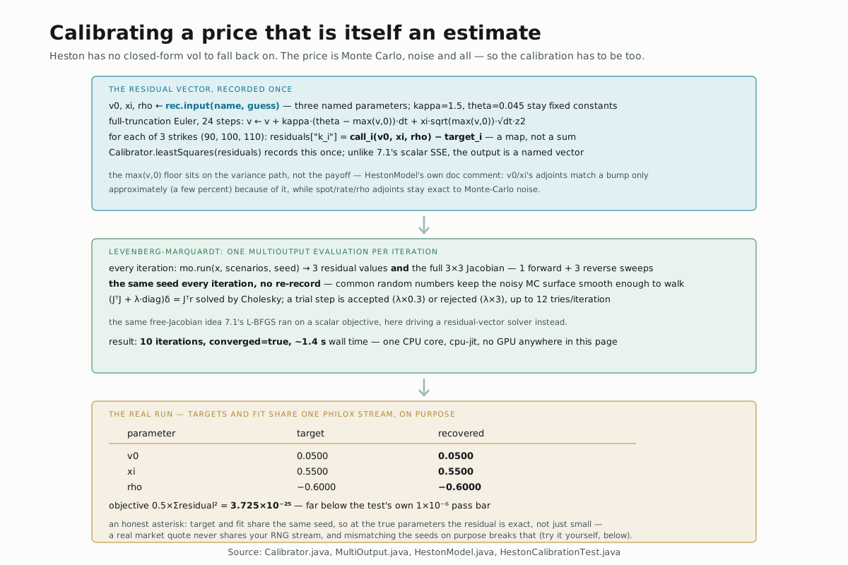
docs/examples/heston-calibration.md states the trick in one line: "the adjoint fixes it: the residual Jacobian is exact for the sampled estimator, and common random numbers make the residual surface smooth enough that Levenberg-Marquardt walks straight to the parameters." Verified directly in Calibrator.evalResiduals: every Levenberg-Marquardt iteration calls mo.run(x, scenarios, seed) with the exact same seed field, regardless of what x is — the random draws never change, only the parameters do. That's the textbook common-random-numbers variance-reduction trick, here applied not to a Greek but to an entire optimizer's convergence.

The residual vector, recorded once

HestonCalibrationTest records three named parameters and a full-truncation Euler path to the option's maturity, then returns a map of residuals — not a single summed number, because Levenberg-Marquardt needs each one separately to build a Jacobian:

Calibrator.Result res = Calibrator.leastSquares(rec -> {
      ADouble v0 = rec.input("v0", 0.03);
      ADouble xi = rec.input("xi", 0.35);
      ADouble rho = rec.input("rho", -0.2);
      Map<String, ADouble> m = hestonMeasures(rec, v0, xi, rho);
      Map<String, ADouble> residuals = new LinkedHashMap<>();
      for (int i = 0; i < STRIKES.length; i++) {
        residuals.put("k" + i, m.get("k" + i).sub(tgt[i]));
      }
      return residuals;
    })
    .parameter("v0", 0.03, 1e-3, 0.5)
    .parameter("xi", 0.35, 1e-2, 3.0)
    .parameter("rho", -0.2, -0.98, 0.5)
    .scenarios(60_000).seed(8675309L)
    .solve();

kappa (mean-reversion speed) and theta (long-run variance) stay fixed constants, the same "hold what you can't identify" move 7.1 made with SABR's beta. The Euler step itself floors the variance at zero every step (vPlus = v.max(0.0), full-truncation) before using it in both the drift and the diffusion — HestonModel.java's own class doc, describing the same scheme mechanically, is explicit that this floor is a real, if small, cost: the v0/xi adjoints match a finite bump only approximately (a few percent) because of it, while the spot/rate/rho adjoints stay exact to Monte-Carlo noise. The floor sits on a measure-zero set in theory, but it's not free.

One MultiOutput evaluation, three residuals and a Jacobian

Calibrator.solveLm builds one MultiOutput over the residual map and reads it, unmodified, every iteration:

Nabla.Valuation v = req.scenarios(scenarios).seed(seed).run();
for (int k = 0; k < res.size(); k++) {
  r[k] = mr.value(res.get(k));
  Map<String, Double> row = mr.gradient(res.get(k));
  for (int i = 0; i < params.size(); i++) {
    j[k][i] = row.getOrDefault(params.get(i).name(), 0.0);
  }
}

One forward sweep plus one reverse sweep per residual — three residuals, so 1 + 3 sweeps total, every iteration, regardless of how close or far the current guess is. That Jacobian feeds a damped Gauss-Newton step, (JᵀJ + λ·diag)δ = Jᵀr, solved by Cholesky; a trial point that lowers the cost is accepted and λ shrinks (more Newton-like), a trial that doesn't is rejected and λ grows (more gradient-descent-like), up to 12 tries per outer iteration. None of that — the Jacobian, the normal equations, the trust-region-style λ schedule — is specific to Heston; it's the general solveLm path 7.1's solveLbfgs sits next to in the same file, chosen automatically by Calibrator.leastSquares(...) instead of Calibrator.of(...).

Did you know?

HestonModel.java is a fully wired, documented, composable Heston step block — it plugs into Nabla.model(HestonMarket, ...) exactly like EquityMarket does, and its own doc comment calls it "Seam 5." HestonCalibrationTest doesn't call it. It hand-rolls the identical full-truncation Euler scheme inline instead, as a private hestonTerminal method. Running both paths side by side, at the same market parameters, same 60,000 scenarios, same seed, confirms they aren't just similar — they're the same computation twice: HestonModel.european and the test's own hestonTerminal both price the K=100 call at exactly 8.874693. The composable class this codebase already built for exactly this purpose sits unused by the one example that needed it.

The real run

Targets are generated at v0=0.05, xi=0.55, rho=−0.6 (kappa=1.5, theta= 0.045 fixed), 3 strikes (90, 100, 110), 60,000 scenarios, seed 8675309, giving real target prices 15.540348, 8.874693, 4.140938. Starting Levenberg-Marquardt from a deliberately wrong guess (v0=0.03, xi=0.35, rho=-0.2):

parameter	target	recovered
v0	0.0500	0.0500
xi	0.5500	0.5500
rho	−0.6000	−0.6000

10 iterations, converged=true, objective (0.5×Σresidual²) 3.725×10⁻²⁷, about 1.4 seconds on one CPU core, cpu-jit. That objective is nine orders of magnitude past the test's own 1×10⁻⁶ pass bar — because the target prices and the calibration objective are built from the same seed, at the true parameters the residual isn't just small, it's an exact replay of the same Philox draws through the same arithmetic, landing at floating-point noise. A real market quote will never hand you that luxury.

Try it yourself

Generate the targets with seed=42 but leave the calibration itself on seed=8675309 — breaking common random numbers on purpose. Predict whether Levenberg-Marquardt still finds (0.05, 0.55, −0.6) before you run it. (It gets close but not exact — v0=0.0522, xi=0.5932, rho=−0.5781 — and hits the 40-iteration cap with converged=false, objective stalled around 6.0×10⁻⁷. Mismatched seeds don't break the fit, but they do put a real floor under how far it can go, one the matched-seed run above never has to face.)

▶️ Run it

No nablatensor-examples showcase runs this calibration standalone — the only place it runs today is the test itself, which isn't tagged or excluded from a plain build, unlike Module 5.1's basket option:

mvn -o -q -pl nablatensor-quant test -Dtest=HestonCalibrationTest

cpu-jit throughout — Calibrator's engine defaults to it and nothing here overrides that default.

⚠️ What this doesn't do

kappa and theta are fixed, not calibrated, the same identifiability shortcut 7.1 took with SABR's beta — Heston's five parameters are no more jointly identifiable from three strikes than SABR's four are from one smile. The near-1e-27 objective above is a demo artifact of matched RNG seeds between target and fit, not a claim about real calibration accuracy; the "try it yourself" section shows the honest floor once that luxury is removed. Twenty-four Euler steps is a coarse discretization with no convergence study run on this page, and nothing here touches a real implied-vol surface, a term structure of maturities, or the full five- parameter joint fit a real desk would eventually need.

What's next

→ Deeper: Calibrate Heston to Monte-Carlo target prices has the full recorded objective this page walks through — its own code sample still writes SDouble, the same stale rename 7.1 already traced through three other files in this engine. → Next: The COS method: calibration without a tape — Module 7.3's answer to the question this page raises but doesn't close: what do you do when the model doesn't fit the tape's primitive op set at all?