The COS method: calibration without a tape
Heston's characteristic function needs sin, cos, and a complex logarithm — none of them tape primitives. This is the one calibration in this section that never touches ADouble, and it's still deterministic and fast.
7.1 and 7.2 both leaned on the same trick: record the model, get an exact
adjoint gradient, hand it to an optimizer. Heston's characteristic function
breaks that trick before it starts — phi(u, T) is built from a complex
square root, a complex exponential, and a complex logarithm, and this
engine's tape has no sin/cos primitive to build any of them from. So the
fastest calibration route for exactly this model can't touch ADouble at
all. What does calibration look like on the other side of that line?
The whole story
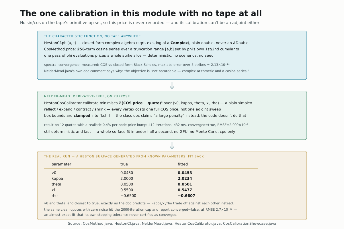
NelderMead.java's own class doc says exactly why this module breaks from
7.1 and 7.2: it's "used to calibrate the COS-priced models (whose objective
is not recordable — complex arithmetic and a cosine series)." Every other
calibration in this Learn section differentiates a recorded tape; this one
minimizes a plain Java function of double[] with a simplex that never asks
for a gradient, because for this particular model there isn't a tape to ask
one of.
A whole strike slice from one set of phi evaluations
HestonCf.phi computes the risk-neutral characteristic function of the
log-return in closed form — square roots, exponentials, and a logarithm, all
on Complex, all plain double underneath:
Complex d = kMinus.mul(kMinus)
    .add(Complex.real(xi * xi).mul(new Complex(u * u, u)))
    .sqrt();
Complex g = kMinus.sub(d).div(kMinus.add(d));
// ...
return c.add(dCoef.mul(v0)).exp();
CosMethod.price turns that into an actual option price by reconstructing
the log-return density as a 256-term cosine series over a truncation range
[a, b] set by phi's own first and second cumulants, then integrating the
payoff against it. Because phi only depends on (u, T), not on strike, one
set of 256 evaluations prices every strike at that maturity — a whole slice
of a smile from one pass, no re-recording, no scenarios, no seed. Against a
closed-form Black-Scholes price at five strikes, the measured gap tops out
at 2.13×10⁻¹⁴ — spectral convergence, not Monte-Carlo noise.
A simplex instead of a sweep
HestonCosCalibrator.calibrate minimizes the sum of squared price residuals
over (v0, kappa, theta, xi, rho) with a plain Nelder-Mead simplex —
reflect, expand, contract, shrink, the textbook four moves, no AadRecorder
anywhere in the file:
java.util.function.ToDoubleFunction<double[]> sse = x -> {
  HestonCf cf = new HestonCf(rate, x[0], x[1], x[2], x[3], x[4]);
  double s = 0.0;
  for (Quote q : quotes) {
    double model = CosMethod.price(cf, OptionType.CALL, spot, q.strike(), rate, q.maturity());
    s += (model - q.price()) * (model - q.price());
  }
  return s;
};
NelderMead.Result nm = NelderMead.minimise(sse, start, step, lo, hi, 2000, 1e-16);
Every simplex vertex costs one full CosMethod.price call per quote — for
this page's 12-quote surface, 12 full price evaluations per vertex, 5+1
vertices per simplex, versus 7.2's 1 + N adjoint sweeps regardless of
quote count. It's the direct trade this page's hook promises: no tape, so
no free gradient, but each individual evaluation is itself so cheap
(closed-form, no Monte-Carlo noise) that the whole thing still finishes in
well under a second. One more thing worth reading in source rather than
trusting the docstring: NelderMead.java's own class comment says out-of-
range points get "a large penalty," but the code doesn't do that anywhere —
clamp() projects every trial point straight onto the box boundary instead.
Run the calibration twice — once against quotes with a realistic 0.4%
per-node price bump, once against noise-free quotes generated by the exact
model being fit — and the noisier run is the one that reports
converged=true. The clean run hits the full 2000-iteration cap with
converged=false, despite landing at RMSE 2.7×10⁻¹², five orders of
magnitude tighter than the noisy run's RMSE 2.0×10⁻². The reason is
sitting in NelderMead's own stopping test:
Math.abs(fv[n] - fv[0]) <= tol * (Math.abs(fv[0]) + tol) with
tol = 1e-16 — once the best function value fv[0] is itself near zero,
that bound becomes an almost impossible target for ordinary simplex
floating-point noise to clear, so an excellent fit can run out the clock
without ever being certified. It's the same shape of gap 6.2's
BermudanLsm hit: a solver's own convergence flag not tracking whether the
answer is actually good.
The real run
CosCalibrationShowcase generates a Heston surface from known parameters
(v0=0.045, kappa=2.0, theta=0.05, xi=0.55, rho=−0.65), applies a
realistic alternating +0.4% price bump to every other quote (12 quotes:
3 maturities × 4 strikes), and fits from a deliberately different start
(v0=0.04, kappa=1.0, theta=0.04, xi=0.3, rho=−0.3):
| parameter | true | fitted |
|---|---|---|
| v0 | 0.0450 | 0.0453 |
| kappa | 2.0000 | 2.0234 |
| theta | 0.0500 | 0.0501 |
| xi | 0.5500 | 0.5477 |
| rho | −0.6500 | −0.6607 |
412 iterations, converged=true, price RMSE 2.009×10⁻², 432 ms, one
CPU core, no GPU, no Monte Carlo anywhere on this page. v0 and theta
land closest to their true values — docs/examples/cos-calibration.md
calls this pair "the well-identified" one — while kappa, xi, and rho
absorb more of the fitting error, trading off against each other exactly as
the same doc predicts.
Try it yourself
CosCalibrationShowcase alternates the per-node bump between 1.0 and
1.004 (+0.4%). Change 1.004 to 1.02 (+2%) and predict how much the
RMSE moves before you run it. (It doesn't stay proportional to the naive
5×: RMSE goes from 2.009×10⁻² to 1.005×10⁻¹, almost exactly 5× worse —
but this time the fit also hits the 2000-iteration cap with
converged=false, and v0/theta are still close to true while kappa
drifts to 2.11 and rho to −0.70, further from true than at 0.4%
noise.)
▶️ Run it
mvn -o -q -pl nablatensor-examples exec:java \
  -Dexec.mainClass=com.nablatensor.examples.CosCalibrationShowcase
Nothing GPU- or engine-related to pass here — CosMethod and NelderMead
never call into the tape or an engine string at all.
⚠️ What this doesn't do
kappa, xi, and rho are recovered far less precisely than v0 and
theta from a single surface — the same identifiability shortfall 7.1 and
7.2 handled by fixing a parameter outright, except this page's fit doesn't
fix anything and just absorbs the ambiguity into three noisier numbers.
CosMethod's truncation range leans entirely on HestonCf's first and
second cumulants (cumulant4 defaults to 0, unused here), which is a
"serviceable approximation" by HestonCf's own comment, not a rigorously
derived bound. And the honest asterisk this page's second sidenote already
raises: converged on a Nelder-Mead result is not a reliable signal of fit
quality in either direction, in this codebase — read the RMSE, not the flag.
What's next
→ Deeper: The COS method: characteristic-function pricing and surface calibration
has the full class table (BsmCf, VarianceGammaCf, and the pinned test
tolerances this page's numbers are checked against).
→ Next: Bootstrapping a curve: zero-rate risk for free —
Module 7.4 leaves single-instrument calibration behind for fitting a whole
multi-curve term structure at once.