Basket options

Everything so far has priced one stock. What happens when the payoff reads three at once — and how much does the correlation between them actually matter?

The whole story

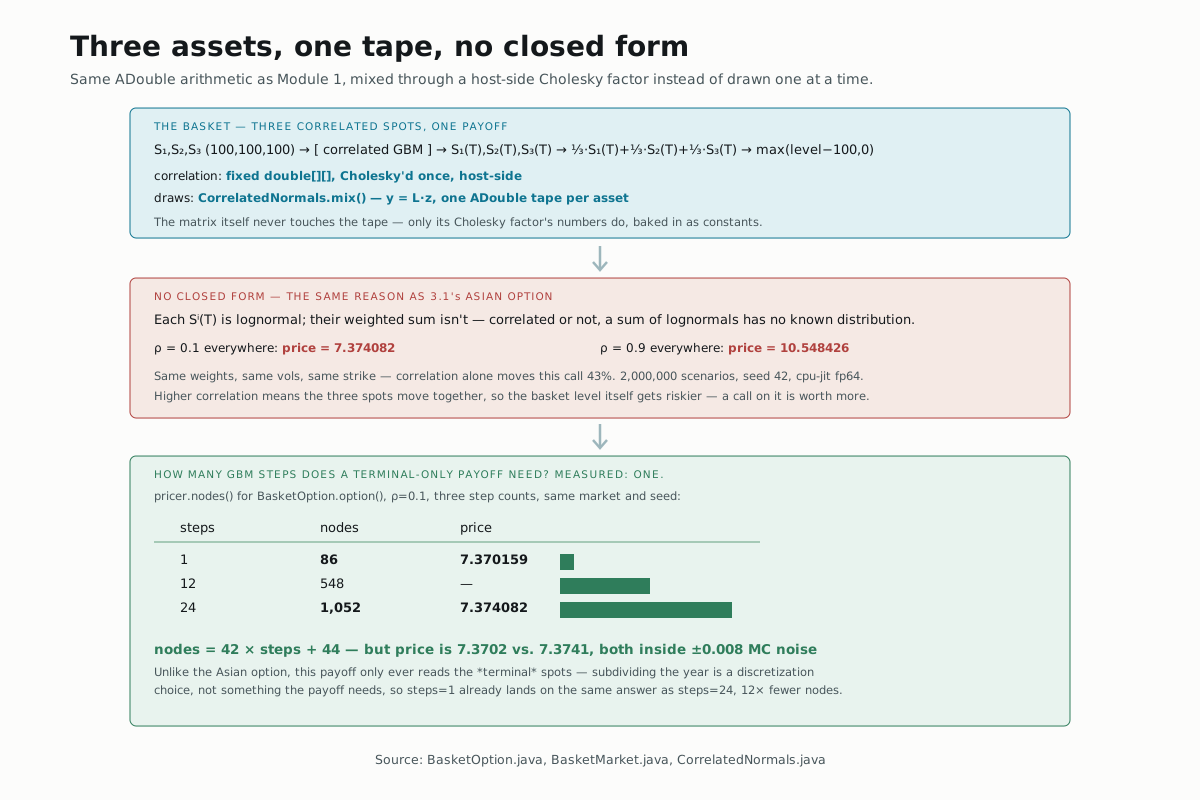
Three correlated spots feed a weighted-sum payoff with no closed form, for the same reason the Asian option has none. Correlation alone moves the price from 7.37 to 10.55. Measuring node counts and prices at steps=1 and steps=24 shows the price barely moves while the tape grows 12×, because this payoff only ever reads the terminal spots.

Did you know?

A basket call has no closed form for the exact same reason 3.1's Asian option doesn't: each of the three spots is lognormal at expiry, but their weighted sum isn't — correlated or not, a sum of lognormal random variables has no known closed-form distribution. Two different modules, one underlying mathematical fact, the same conclusion: reach for Monte Carlo.

One product, three spots

BasketOption.option looks almost exactly like Products.european from Module 1, except every ADouble operation on the spot happens three times — once per asset — and the correlation between the three GBM paths is mixed in before the drift is even applied:

CorrelatedNormals mixer = CorrelatedNormals.of(corr);
...
for (int t = 0; t < steps; t++) {
  ADouble[] z = mixer.draw(rec);
  for (int i = 0; i < ASSETS; i++) {
    s[i] = s[i].mul(drift[i].add(vol[i].mul(sqrtDt).mul(z[i])).exp());
  }
}
ADouble level = rec.constant(0.0);
for (int i = 0; i < ASSETS; i++) {
  level = level.add(s[i].mul(weights[i]));
}

weights and corr are plain double[]/double[][] arguments, not market inputs — a bank doesn't hedge a correlation assumption the way it hedges a spot, so there is nothing to differentiate there. Only s1/s2/s3, v1/v2/v3, and rate — BasketMarket's seven record components — are ADoubles on the tape.

Did you know?

CorrelatedNormals.of(corr) runs a Cholesky factorization in plain Java, once, before a single tape node exists — its own doc comment says so directly: "the factor is computed once at record time... the per-step mixing is a handful of primitive nodes." The 3×3 correlation matrix itself never touches the adjoint tape; only the nine numbers in its Cholesky factor do, baked in as constants that mixer.draw(rec) multiplies against fresh rec.randn() draws every step.

What correlation is worth

BasketMarket.equalWeighted() (spots 100/100/100, vols 20%/25%/30%, rate 2%) priced with equal 1/3 weights, a 100 strike, and 24 GBM steps, under two correlation matrices — everything pairwise 0.1, and everything pairwise 0.9 — 2,000,000 scenarios, seed 42, cpu-jit, fp64:

pairwise ρ	price
0.1	7.374082
0.9	10.548426

Nothing else changed — same spots, same vols, same weights, same strike. Correlation alone moved this call's price by 43%. That's the whole reason corr exists as an argument at all: when the three names move together, the basket level itself gets riskier, and a call on a riskier level is worth more.

How many steps does this actually need?

BasketOption.option's steps parameter subdivides the year into GBM sub-steps, the same way Products.asian's fixing count did in 3.1. Building the ρ=0.1 basket at three step counts and reading pricer.nodes():

steps	nodes
1	86
12	548
24	1,052

That's nodes = 42 × steps + 44 at every point — 42 new nodes per step (a fresh correlated draw for each of the three assets, plus one GBM update per asset), on top of 44 fixed nodes for the market inputs, the weighted sum, and the payoff.

But watch what happens to the price, not just the tape, at steps=1 versus steps=24, same market, same seed:

steps	nodes	price
1	86	7.370159
24	1,052	7.374082

7.3702 versus 7.3741 — both inside the run's own Monte-Carlo standard error (±0.0078). Unlike the Asian option, this payoff never reads an intermediate spot; level only ever uses s[i] after the loop finishes. Subdividing the year is a discretization choice, not something the payoff demands — a constant-volatility GBM can be sampled exactly in one jump from 0 to T. steps=1 already lands on the same answer as steps=24, for 12× fewer nodes.

Did you know?

This is the opposite lesson from 3.1's Asian option, and it's worth noticing precisely because the code looks the same — a loop over steps calling the same GBM update. The Asian payoff reads every intermediate path value and sums it, so its fixing count is part of the contract's definition and the tape genuinely needs all 252 of them. The basket payoff only ever reads the final s[i], so its step count is pure numerical convention — a knob you could turn down to 1 without changing what you're computing, only how many nodes it costs to compute it.

Try it yourself

Change the two correlation matrices to something asymmetric — say ρ(1,2)=0.9 but ρ(1,3)=ρ(2,3)=0.1 — and reprice. The basket level now depends on which two names move together, not just how correlated the basket is "on average"; CorrelatedNormals.of will throw IllegalArgumentException instead of a wrong number if you accidentally hand it a matrix that isn't positive definite, which is an easy mistake once the three pairwise correlations stop being equal.

▶️ Run it

mvn -o -q -pl nablatensor-quant test -P mc \
  -Dtest=BasketAndCurveTest#basketDeltasMatchBumpAndRisePriceWithCorrelation

-P mc is required: the pom tags this test mc (Monte-Carlo validation, slower than the default suite) and excludes it from a plain mvn test by default. It only exercises cpu-jit, so nothing here touches a GPU backend.

⚠️ What this doesn't do

There is no nablatensor-examples showcase for the basket yet — the only place this code runs today is BasketAndCurveTest, which is why "Run it" points at a test instead of a Products-style demo class with a printed table. It also fixes the basket at exactly three assets (BasketOption.ASSETS = 3, checked at record time) rather than an arbitrary N, and doesn't cover a spread option — a payoff on the difference between two assets instead of their weighted sum, which needs its own closed-form comparison. That's next.

What's next

→ Deeper: CorrelatedNormals.java has the full Cholesky mixing, including the 2×2 pair(rho) shortcut this page's basket didn't need. → Next: Spread options — Kirk vs. Margrabe vs. Monte Carlo, where two assets and a closed-form approximation replace three assets and none.