Spread options — Kirk vs. Margrabe vs. Monte Carlo

A gas-fired power plant's profit isn't the price of electricity, and it isn't the price of gas — it's the difference between the two. How do you price an option on that difference, when there are two different closed-form answers on offer and neither one is exact?

The whole story

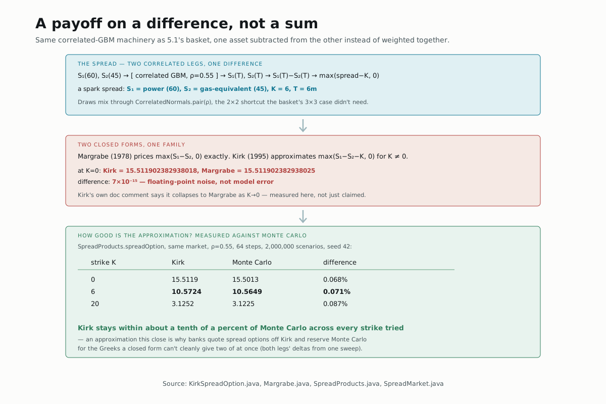
Two correlated GBM legs feed a payoff on their difference instead of their sum. Margrabe's exact formula and Kirk's approximation are the same family — Kirk collapses to Margrabe at zero strike, measured to 7e-15. Kirk stays within about a tenth of a percent of Monte Carlo across every strike tried.

Did you know?

KirkSpreadOption's own doc comment says it "collapses to the exact Margrabe price" as the strike goes to zero — and that's not a hand-wavy claim. Pricing the same market at K=0 through both formulas gives 15.511902382938018 (Kirk) and 15.511902382938025 (Margrabe): a difference of 7×10⁻¹⁵, which is floating-point rounding noise, not model error. Two formulas published seventeen years apart (Margrabe 1978, Kirk 1995) turn out to be the exact same function at one boundary.

Two legs, one difference

SpreadProducts.spread looks almost like 5.1's BasketOption.option, except it stops at two assets and subtracts instead of summing — and it reaches for CorrelatedNormals.pair(rho), the 2×2 shortcut whose full 3×3 sibling the basket already used:

CorrelatedNormals mix = CorrelatedNormals.pair(rho);
...
for (int t = 0; t < steps; t++) {
  ADouble[] z = mix.draw(rec);
  s1 = s1.mul(drift1.add(v1.mul(sqrtDt).mul(z[0])).exp());
  s2 = s2.mul(drift2.add(v2.mul(sqrtDt).mul(z[1])).exp());
}
ADouble spread = s1.sub(s2);
ADouble intrinsic = spread.sub(strike).max(0.0);

SpreadMarket's seven components include a carry (yield1/yield2) for each leg instead of a single shared one — commodities have a convenience yield the way equities have a dividend yield, and KirkSpreadOption and Margrabe both take it as a per-leg input for exactly that reason. SpreadMarket.sparkSpread() sets both to zero and leans on the spot gap (60 vs. 45) to stand in for "power costs more per unit than the gas needed to make it," which is what a real spark spread actually is: the heat-rate margin a gas plant earns, priced as an option on a difference.

Two closed forms for the same idea

Margrabe (1978) prices max(S1 − S2, 0) exactly — no strike, so it's the option to exchange one asset for another. Kirk (1995) extends that to a nonzero strike by treating the spread as an exchange between F1 and F2 + K, folding the strike into an effective volatility that blends vol1, vol2, and how far F2 + K sits from F2:

double a = f2 / (f2 + strike);
double sigma = Math.sqrt(vol1 * vol1 - 2.0 * rho * vol1 * vol2 * a + vol2 * vol2 * a * a);

At strike = 0, a = 1 and this collapses algebraically to Margrabe's own sqrt(vol1² + vol2² − 2ρ·vol1·vol2) — which is exactly the 7×10⁻¹⁵ match above, not a coincidence.

How good is the approximation?

SparkSpreadShowcase's market (power spot 60, gas-equivalent 45, both vols 35%/30%, ρ=0.55, 6 months) priced by Kirk and by SpreadProducts.spreadOption at 64 steps, 2,000,000 scenarios, seed 42, cpu-jit, fp64, across three strikes:

strike K	Kirk	Monte Carlo	difference
0	15.5119	15.5013	0.068%
6	10.5724	10.5649	0.071%
20	3.1252	3.1225	0.087%

Kirk stays within about a tenth of a percent of the Monte-Carlo price at every strike tried. That's close enough that a desk quotes spread options off Kirk directly and reserves Monte Carlo for the one thing the closed form can't cleanly give: both legs' deltas from a single sweep. SparkSpreadShowcase's own adjoint run reports dS1 = +0.8099 and dS2 = −0.7453 at K=6 — long the first leg, short the second, from the one .greeks() call.

Did you know?

Correlation cuts the opposite way here from 5.1's basket. A basket call is a call on a sum, so it gets more valuable as the names move together — 5.1 measured a 43% jump from ρ=0.1 to ρ=0.9. A spread option is a call on a difference, so it gets more valuable as the names move apart: at this same market, Kirk gives 10.5724 at ρ=0.55, 12.3121 at ρ=0, and 13.7377 at ρ=−0.55. Same mathematical machinery — a Cholesky mix of two correlated normals — pointed at a sum in one module and a difference in the next, with the correlation sensitivity flipping sign because of it.

Both legs here also only ever get read after the step loop finishes, the same as 5.1's basket — so the same discretization-doesn't-matter property holds. nodes() at steps=1 is 56, at steps=64 is 1,631 (nodes = 25 × steps + 31), and the two prices land close together — 10.5800 at steps=1 versus 10.5649 at steps=64, both within roughly two Monte-Carlo standard errors of each other (±0.0077 each) — for 29× fewer nodes.

Try it yourself

Using the ρ=0.55/0/−0.55 numbers above, predict what Kirk gives at ρ=−0.9 before running it: the trend keeps climbing, since the two legs are now diverging even harder — you should land somewhere past 13.74, closer to the ρ→−1 limit where the spread's effective volatility approaches vol1 + vol2.

▶️ Run it

mvn -o -q -pl nablatensor-examples exec:java \
  -Dexec.mainClass=com.nablatensor.examples.SparkSpreadShowcase

Runs on cpu-jit only. The same command also prints a Schwartz one-factor futures curve with a seasonality overlay — that's commodity mean-reversion, a different model family entirely, out of scope for this page.

⚠️ What this doesn't do

Kirk is an approximation, not a closed form the way Margrabe is — accurate to a tenth of a percent here, but that error grows for wider vols or more extreme strikes than this page tried, which is exactly why the Monte Carlo path exists alongside it rather than instead of it. This page also doesn't cover the Schwartz mean-reverting model SparkSpreadShowcase prints alongside it (commodity prices don't follow GBM the way equities do — a separate topic), or a spread on more than two legs, which would need BasketOption's three-asset machinery with a difference instead of a weighted sum, and isn't something this codebase currently offers.

What's next

→ Deeper: Commodity models and spread options covers the Schwartz one-factor model and seasonality overlay this page skipped, plus the full pinned-test tolerances (Kirk vs. Monte Carlo to 3%, exchange option to 2%, adjoint deltas vs. bump to 5e-3). → Next: Quanto and convexity adjustments — the adjustment a cross-currency payoff needs, falling out of the same tape for free.