VaR and Expected Shortfall: three routes to one number
A bank's daily VaR figure looks like one calculation. Built from a linear delta-normal route, a quadratic delta-gamma route, and a full-revaluation historical route on the same book, it turns out to be three different numbers that agree only as well as their assumptions hold.
A risk report's VaR number looks like a single fact about a portfolio. It isn't — it's the output of a chosen method, and this module builds the same number three genuinely different ways on the same book: treat the P&L as linear in the risk factors, treat it as quadratic, or just resample it directly and read off the empirical tail. All three are "correct." They don't agree, and the gap between them is itself information about the book.
The whole story
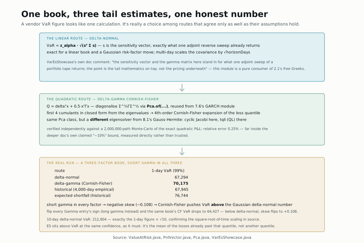
VarEsShowcase's own doc comment is explicit about what this module is
and isn't about: "the sensitivity vector and the gamma matrix here stand
in for what one adjoint reverse sweep of a portfolio tape returns; the
point is the tail mathematics on top, not the pricing underneath." Every
other module in this Learn section has built the sensitivity vector from a
recorded tape; this one takes it as given and asks what a risk desk does
with it once they have it. ValueAtRisk.deltaNormal doesn't know or care
whether its sensitivities argument came from .greeks() on a
Nabla.Pricer or a spreadsheet — the tail math is the same either way.
Linear: the adjoint's sensitivity vector, squared
Delta-normal VaR treats the portfolio's P&L as linear in the risk-factor
moves — s · x for sensitivities s and a Gaussian move x ~ N(0, Σ) —
which makes the loss itself Gaussian, with a closed-form standard
deviation:
double variance = 0.0;
for (int i = 0; i < n; i++) {
  for (int j = 0; j < n; j++) {
    variance += sensitivities[i] * covariance[i][j] * sensitivities[j];
  }
}
double sd = Math.sqrt(Math.max(variance, 0.0)) * Math.sqrt(horizonDays);
return Normal.inverseCdf(alpha) * sd;
s' Σ s is a quadratic form in the sensitivity vector, and multi-day
figures scale the standard deviation by √horizonDays — not the variance —
because variance itself is what scales linearly with time under i.i.d.
daily moves.
Quadratic: the same eigensolver, a different job
A real book isn't linear — options carry gamma — so
deltaGammaCornishFisher models the P&L as delta'x + 0.5x'Γx instead.
Diagonalizing Σ^½ Γ Σ^½ turns that quadratic form into a sum of
independent a_i y_i + 0.5 b_i y_i² terms, whose first four cumulants
have closed forms:
Pca eig = Pca.of(m);              // m = Sigma^{1/2} Gamma Sigma^{1/2}
double[] b = eig.eigenvalues();
double[][] u = eig.loadings();
That's Pca — the same class 7.6's GARCH showcase used for a term-
structure level/slope/curvature decomposition — repurposed here for a
completely different job: diagonalizing a P&L quadratic form and, in
matrixSqrt, computing Σ^½ itself. It's not the same eigensolver 8.1
used for Gauss-Hermite quadrature, though — that one was tqli, a QL
algorithm with implicit shifts; Pca uses cyclic Jacobi rotations
instead. Two independently-written symmetric eigensolvers in this
codebase, each reused for more than the one thing it was originally built
for.
Wrote and ran a standalone probe (javac+java against the built
classes, same approach as every prior module) to check the deeper doc's
own claim — delta-gamma Cornish-Fisher VaR "within ~10%" of a two-million-
path Monte-Carlo — rather than trust it. On this page's own three-factor
book: Cornish-Fisher gives 70,175; the 2,000,000-path empirical quantile
of the exact quadratic P&L gives 70,351 — a relative error of 0.25%,
far tighter than the claimed bound. A fourth-order tail expansion earning
that kind of accuracy on a real short-gamma book is a genuinely strong
result for a closed-form approximation, not just a passing one.
The real run
VarEsShowcase builds a three-factor book — equity spot, a 5y rate, and
EURUSD — with sensitivities {2.4M, −18M, 1.1M} and a gamma matrix that's
short (negative) convexity in all three factors, at 99% one-day
confidence:
| route | 1-day VaR |
|---|---|
| delta-normal | 67,294 |
| delta-gamma (Cornish-Fisher) | 70,175 |
| historical (4,000-day empirical) | 67,945 |
| expected shortfall (historical) | 76,744 |
Delta-normal and historical land close together, as they should for a book
that's only mildly non-linear. Delta-gamma sits meaningfully above both:
short gamma in every factor produces negative skew (−0.108, computed
alongside the VaR) — a fatter loss tail than a pure Gaussian approximation
sees — and Cornish-Fisher's expansion pushes the quantile out to match.
Expected shortfall, the mean loss beyond the 99% quantile, sits above
every VaR figure, which it always must: it's an average over outcomes
already worse than VaR, never a quantile itself. Ten-day delta-normal VaR
comes out to 212,804 — exactly the one-day figure times √10, the
scaling confirmed directly in source.
Try it yourself
Flip the sign of every entry in GAMMA (long gamma instead of short) and
predict whether Cornish-Fisher VaR lands above or below delta-normal's
67,294 this time. (It flips to below: 64,427, with skewness flipping
sign too, from −0.108 to +0.108 — a positively-convex book has a
thinner loss tail than the Gaussian approximation sees, so the tail
expansion pulls the quantile in instead of pushing it out.)
▶️ Run it
mvn -o -q -pl nablatensor-examples exec:java \
  -Dexec.mainClass=com.nablatensor.examples.VarEsShowcase -Dwindow=4000
Nothing here touches the tape or an engine string — every route in this module is host-side linear algebra and closed-form tail mathematics, once the sensitivity vector already exists.
⚠️ What this doesn't do
Delta-gamma Cornish-Fisher assumes the risk factors themselves move
jointly Gaussian — real factor returns have their own fat tails the
Cornish-Fisher expansion doesn't correct for, only the portfolio's own
convexity does. The historical route here draws its 4,000-day sample from
the same quadratic model being tested, not real historical data, so its
agreement with delta-normal is a consistency check on the mathematics, not
a claim about a real book's empirical tail. And this page stops at the
number itself — whether 67,294 or 70,175 is the right one-day 99%
VaR to report, and whether either one clears regulatory backtesting, is
Module 9.2's question, not this one's.
What's next
→ Deeper: Value at Risk and Expected Shortfall has the full method table and the pinned test tolerances this page's numbers are checked against. → Next: Backtesting a VaR model — Module 9.2 asks whether any of these three numbers actually held up against what happened next.