Replaying it
MonteCarlo.of(...).on("cpu-jit").build() turns Products.europeanCall() into a price and every Greek, checked against Black-Scholes, from one recorded tape.
You've recorded a tape. Nobody's paid for anything yet — a tape is just a
recipe. What does it take to turn (x+2)*x-shaped recording into an actual
option price, with delta, vega, and rho included, and no separate run for
each one?
The whole story
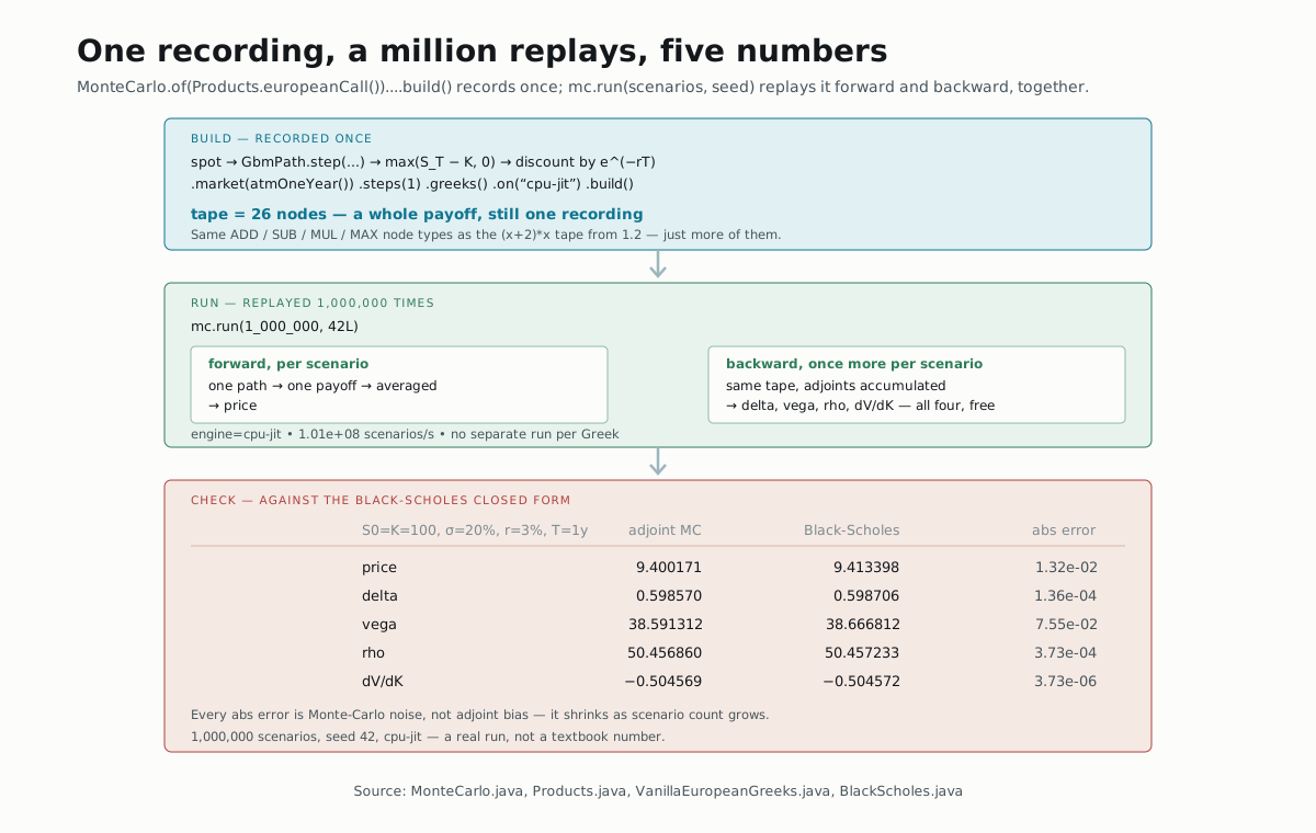
The gradient mc.run(...) hands back is an EquityMarket — the exact same
record type as the market you priced against. EquityMarket.spot() carries
delta, vol() carries vega, rate() carries rho, strike() the strike
sensitivity: the engine reuses the market's own shape as the shape of its
gradient, so p.greek(EquityMarket::spot) is really just "the sensitivity to
the field named spot."
Building the pricer
Everything from 1.2 was one lambda, one small tape, no finance. This is the
same AadRecorder.record(...) machinery, pointed at a real payoff instead:
EquityMarket market = EquityMarket.atmOneYear();   // S0=K=100, sigma=20%, r=3%, T=1y

try (MonteCarlo<EquityMarket> mc = MonteCarlo.of(Products.europeanCall())
    .market(market)
    .steps(1)          // the terminal value is all a European needs
    .fp64()
    .greeks()
    .on("cpu-jit")     // plain Java: no native lib, no incubator flag
    .build()) {
  ...
}
.build() is the record step from 1.2, just wearing a builder: it calls
Products.europeanCall()'s own record(rec, in, grid) exactly once and
gets back a tape, the same way AadRecorder.record(...) did.
What actually got recorded
Products.europeanCall() is a handful of ADouble operations, the same
kind 1.1 and 1.2 already covered — just walking a simulated path instead of
one line:
public static Product<EquityMarket> european(OptionType type) {
  return new Named("European " + type, (rec, in, grid) -> {
    Sim sim = new Sim(rec, in, grid);
    ADouble terminal = sim.spot;
    for (int t = 0; t < grid.steps(); t++) {
      terminal = sim.model.step(terminal, rec.randn(), t);
    }
    rec.output(sim.discount(intrinsic(type, terminal, sim.strike)));
  });
}
One step (grid.steps() == 1, from .steps(1)), one randn() draw, a
max(S_T − K, 0) (intrinsic), and a discount factor. Recorded, this comes
to exactly 26 nodes — small enough to read by hand, the same struct-of-
arrays shape as 1.2's four-node tape, just longer.
Running it
mc.run(scenarios, seed) is the replay step — forward once per scenario for
the price, backward once per scenario for every Greek, in the same pass:
Nabla.TypedValuation<EquityMarket> p = mc.run(1_000_000, 42L);
BlackScholes bs = BlackScholes.of(OptionType.CALL, market);

p.price();                       // 9.400171
p.greek(EquityMarket::spot);     // delta:  0.598570
p.greek(EquityMarket::vol);      // vega:  38.591312
p.greek(EquityMarket::rate);     // rho:   50.456860
p.greek(EquityMarket::strike);   // dV/dK: -0.504569
That's a real run: engine=cpu-jit tape=26 nodes, 1,000,000 scenarios at
1.01×10⁸ scenarios/s, checked against BlackScholes.of(OptionType.CALL, market) — the closed-form reference. Every one of the five numbers above
lands within Monte-Carlo noise of Black-Scholes, exactly as the figure
shows.
mc is still open after that call — a MonteCarlo isn't a one-shot script,
it's a compiled kernel you can reuse. mc.run(mc.market().withSpot(101.0), 1_000_000, 42L) reprices under a bumped market on the same tape, no
re-recording and no rebuilding — straight from MonteCarlo's own class doc.
That's what "record once, replay many" means in practice: the many can be
many scenarios, or many markets, on the same recording.
Try it yourself
Swap Products.europeanCall() for Products.europeanPut(), and
BlackScholes.of(OptionType.CALL, market) for BlackScholes.of(OptionType.PUT, market). Guess the sign of p.greek(EquityMarket::spot) before you check —
a put loses value as the underlying rises, so delta should come back
negative this time.
▶️ Run it
mvn -o -q install
mvn -o -q -pl nablatensor-examples exec:java \
  -Dexec.mainClass=com.nablatensor.examples.VanillaEuropeanGreeks \
  -Dscenarios=1000000
That's the exact command behind the numbers above — cpu-jit, 1,000,000
scenarios, seed 42 by default. No GPU backend involved.
⚠️ What this doesn't do
This is the smallest payoff that touches real finance: one time step, one
underlying, a European exercise. It doesn't show what happens when a payoff
needs the whole path (Module 3), what it costs to add ten more risk
factors to the market record (nothing — Module 2 is the actual side-by-side
against bump-and-revalue), or what changes if you swap "cpu-jit" for a GPU
backend (Module 4). And nobody has checked whether this price is fast yet
— just that it's correct.
What's next
→ Deeper: Vanilla European option Greeks in Java
is the technical version of this page — note its code sample predates the
Nabla.TypedValuation/.greek(EquityMarket::spot) API this page uses; the
mechanics and the market are the same.
→ Next: Adjoint vs. bump-and-revalue, side by side,
where the same reverse sweep is timed against the classic finite-difference
alternative — the README's headline benchmark, walked through step by step.