Adjoint vs. bump-and-revalue, side by side

Module 1 got you delta, vega, rho, and a strike sensitivity from one call to run(). How else would you even get those four numbers — and what would it cost?

The whole story

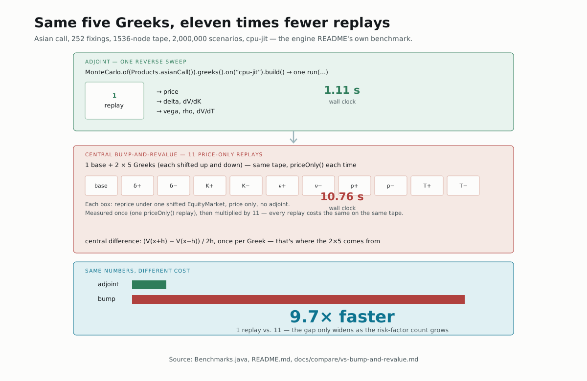
One adjoint reverse sweep produces price plus five Greeks in 1.11 seconds. Central bump-and-revalue reprices the same tape eleven times — a base valuation plus an up and down shift for each of five Greeks — in 10.76 seconds. Same numbers, 9.7 times slower, and the gap widens as the risk-factor count grows.

Did you know?

This benchmark switches from 1.3's European call to Products.asianCall() — 252 daily fixings instead of one time step — on purpose. Products.european's 26-node tape from Module 1 is so cheap that adjoint and bump would look nearly identical; the Asian call's 1,536-node tape is what makes an 11×-vs-1× cost difference actually show up in wall-clock seconds instead of noise. (The payoff itself is Module 3 — for now, treat it as "a bigger tape.")

The classic alternative: bump-and-revalue

A central difference estimates one Greek by nudging one input and repricing twice: (V(x+h) − V(x−h)) / 2h. Benchmarks.java needs five Greeks — delta, dV/dK, vega, rho, dV/dT — so that's 1 base valuation plus 2 × 5 shifted ones, eleven price-only Monte Carlo runs for the same information one adjoint sweep gives you in one:

private static final int GREEKS = 5;   // delta, dV/dK, vega, rho, dV/dT

double oneRevalSec = bestOf(3, () -> priceOnly.run(scenarios, seed).seconds());
double bumpSec = (1 + 2 * GREEKS) * oneRevalSec;

Notice what that second line does not do: it doesn't actually build ten shifted EquityMarkets and reprice under each one. It times a single priceOnly() replay and multiplies by eleven — a fair shortcut, not a fudge, because 1.3's second sidenote already showed that swapping the market on a built kernel costs exactly what the original run cost. Eleven replays of the same tape really do cost eleven times one.

Timing the adjoint sweep

The adjoint side is a single MonteCarlo built with .greeks() instead of .priceOnly() — same product, same market, same tape shape as 1.3, just Asian instead of European:

double adjointSec = bestOf(3, () -> adjoint.run(scenarios, seed).seconds());

adjoint: price=5.301676 delta=0.561932 vega=22.389375 rho=23.603735

That's a real, checked run — docs/compare/vs-bump-and-revalue.md cites the same numbers, reconciled against the closed form the same way 1.3's page was. Put the two timings side by side and the table from the whole-story picture falls out directly:

method	replays	wall clock	speedup
adjoint — value + 5 Greeks, one reverse sweep	1	1.11 s	9.7×
central bump — 1 + 2×5 price-only revaluations	11	10.76 s	1.0×

Did you know?

That 9.7× isn't the ceiling — it's just what five Greeks happens to cost. bumpSec scales as 1 + 2N; adjointSec doesn't have an N in it at all. docs/compare/vs-bump-and-revalue.md spells out the next step: at N = 20 risk factors, bump-and-revalue needs 41 revaluations against the same single adjoint sweep. A real bank's risk book has far more than 20 factors — which is the actual reason adjoint AD exists, not just a Java performance trick.

Try it yourself

GREEKS is a plain int at the top of Benchmarks.java. Without changing anything else, work out by hand what bumpSec's multiplier becomes for a book with 20 risk factors (1 + 2×20 = 41) versus 100 (1 + 2×100 = 201). adjointSec's multiplier is 1, unconditionally, at every one of those sizes.

▶️ Run it

mvn -o -q install
mvn -o -q -pl nablatensor-examples exec:java \
  -Dexec.mainClass=com.nablatensor.bench.Benchmarks \
  -Dscenarios=2000000 -Dsteps=252

This prints the table above, then a second "backend matrix" table — every engine referential machine can run, same tape, scenarios per second. That second table is Module 4's topic; ignore it for now. (The class's own doc comment says -pl nablatensor-bench — there's no such module in this repo; the command above, straight from the README, is the one that actually works.)

⚠️ What this doesn't do

This page only explains the top half of Benchmarks.java's output — the backend matrix underneath it is Module 4. It doesn't explain what an Asian option's payoff actually computes (Module 3), and the wall-clock numbers are specific to one 16-vCPU machine — the README says so itself: "your numbers will differ." What won't differ is the shape of the two formulas: 1 versus 1 + 2N.

What's next

→ Deeper: NablaTensor vs bump-and-revalue has the full method section and the N = 20 projection this page only summarized. → Next: Reading a Greek you didn't ask for, where each of .greek(EquityMarket::spot)'s siblings actually comes from in the reverse sweep.