CVA from first principles
10.3 took a CVA sensitivity vector as given. Where does the CVA number underneath it actually come from? A Monte-Carlo integral over expected exposure and default probability, recorded once on the adjoint tape — and a real, verified gap between the counterparty curve the demo prints and the one it actually prices with.
10.3 handed you a CVA sensitivity vector and built a capital charge out of it. Where does the CVA number underneath that vector actually come from? An integral over a counterparty's expected exposure and default probability, simulated on a time grid and recorded once, the same way every other page in this Learn section has recorded a valuation.
The whole story
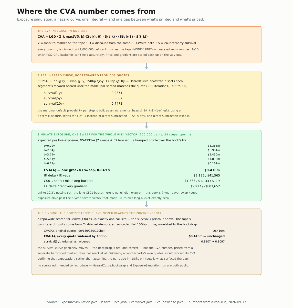
Every quantity here — mark-to-market, exposure, the CVA integrand — is
divided by MONEY_UNIT = 1,000,000 before it ever touches the tape.
ExposureSimulation's own doc comment explains why: unscaled sums run
past 1e10 in reporting-currency terms, "the difference between a
stable and an unusable single-precision replay." Divide down to O(1)
quantities, replay, then scale the price and gradient back up on the way
out — the same trick that keeps this exact tape usable on cpu-jit's
fp64 and a GPU backend's fp32 without two different implementations.
The CVA integral, in one line
CVA = LGD * sum_k max(V(t_k) - C(t_k), 0) * D(t_k) * ( S(t_{k-1}) - S(t_k) )
Three ingredients, each already familiar from earlier chapters: V is a
mark-to-market recorded the same way every option in this Learn section
has been (here, two interest-rate swaps and an FX forward, summed);
D is a discount factor off the same Hull-White path driving the trade
values; S is the counterparty's survival probability, and its drop
between two dates is the chance of default arriving exactly then.
Build a real hazard curve from CDS quotes
HazardCurve.bootstrap strips a piecewise-flat forward hazard from
ascending CDS quotes, one segment at a time, by bisection:
double target = quote.parSpread();
for (int iteration = 0; iteration < 200; iteration++) {
  double mid = 0.5 * (lo + hi);
  hazards[segment] = mid;
  double modelSpread = parSpread(knots, hazards, segment + 1, lgd, discount);
  if (modelSpread > target) { hi = mid; } else { lo = mid; }
}
Fed counterparty A's real quotes — 90bp at 1y, 130bp at 3y, 150bp
at 5y, 170bp at 10y — this gives real survival numbers:
survival(1y) = 0.9851, survival(5y) = 0.8807, survival(10y) = 0.7473. The marginal default probability each step needs is built as an
incremental hazard, S(t_{k-1}) · (1 - e^{-Δλ}), using a six-term
Maclaurin series for 1 - e^{-x} instead of direct subtraction — Δλ
is tiny at every step, and 1.0 - Math.exp(-x) for small x throws away
almost every significant digit to cancellation before the series ever
gets a chance to.
Simulate exposure, one sweep for the whole risk vector
A recorded Hull-White short rate and a lognormal FX spot drive every
trade's mark-to-market at every grid date; one .greeks() run returns
the CVA number and its complete gradient:
Nabla.TypedPricer<CvaMarket> pricer =
    (useFp64() ? model.fp64() : model.fp32()).greeks().on(engine).build();
Real numbers, 200,000 paths, 24 steps, cpu-jit, netting set NS-CPTY-A
(a 7-year payer swap, a 5-year receiver, an FX forward): the expected
positive exposure profile peaks early, $8.385m at t=0.29y, and runs
off toward zero as trades mature, $0.167m at t=6.71y — a real, humped
shape, not asserted. CVA(A) = $0.410m, from one sweep in 0.849 s.
The same sweep also gives IR delta ($2,185) and vega ($41,565), CS01
by tenor bucket ($1,338 / $1,133 / $119 short/mid/long), FX delta
($9,917), and a recovery gradient (-$683,652) — no second run for any
of them.
Unlike 10.3's netting set, the long CS01 bucket here is genuinely
nonzero. 10.3's book matured at 5 years, so its hazard curve's 7.5-year
vertex never touched any real exposure. This book's 7-year payer swap
keeps exposure alive past that point, and the long bucket, $119, proves
it.
A repo-wide search for .curve() — the accessor onto the bootstrapped
HazardCurve above — turns up exactly one call site in the entire
nablatensor-cva module and its examples: the survival() printout in
CvaShowcase.main()'s [1/8] section. The Monte-Carlo integral's own
hazard inputs (CvaMarket::hazardShort/hazardMid/hazardLong) come from
a completely separate object, CvaMarket.demo() — a hardcoded flat
150bp curve, unrelated to whichever counterparty's HazardCurve gets
bootstrapped and printed alongside it. The bootstrap is real; it just
never reaches the kernel that prices the trade.
Try it yourself
If the counterparty's own CDS quotes actually drove the CVA number, a
credit deterioration — every quote widened by 100bp — should make CVA
worse. Bootstrapped a second curve from 190/230/250/270bp quotes,
attached it to the same counterparty, and reran ExposureSimulation
against it. Real numbers: survival(5y) genuinely moves, 0.8807 to
0.8097 — the bootstrap reacted exactly as it should. CVA(A) does not
move at all: $0.410m, unchanged to the last printed digit. Predicting
otherwise, then checking, is what surfaces the gap the sidenote above
names — no source edit needed, both HazardCurve.bootstrap and
ExposureSimulation.run are already public.
▶️ Run it
The same netting set, live: build the Hull-White-plus-FX tape, read the
whole CVA risk vector off one adjoint sweep, then bootstrap a real hazard
curve and watch survival move while CVA doesn't — right here, in your
browser through TeaVM, on a
stand-in for the real ExposureSimulation rewritten around chapter 1.3's
cell's own limitation, rec.input() directly instead of Nabla.Inputs <CvaMarket>'s reflection layer. HazardCurve.bootstrap runs completely
unmodified. The browser cell uses 2,000 paths × 8 steps so the full showcase
finishes in a browser; the Maven command below retains the 200,000 × 24 defaults:
Or run the real thing:
mvn -o -q install
mvn -o -q -pl nablatensor-examples exec:java \
  -Dexec.mainClass=com.nablatensor.examples.CvaShowcase
Defaults to cpu-jit, 200,000 paths, 24 steps, no GPU. This runs the
full 8-stage showcase — netting sets through the three PRA methods —
this page only walked stages [1/8]–[3/8]; 10.3 already covered the
SA-CVA aggregation stages, and BA-CVA/the PRA methods are Chapter 11.3's.
⚠️ What this doesn't do
The hazard-curve gap above is worth stating plainly rather than papering
over: CvaMarket.demo()'s flat 150bp curve means every counterparty
in every showcase this Learn section has used — A's real term structure,
B's flat 110bp curve alike — gets priced against the identical hazard
level, regardless of which HazardCurve object sits on its CreditName.
The printed [1/8] survival numbers are real and correctly bootstrapped;
they just describe a curve the pricing engine never sees. Everything
else stays scoped as before: one netting set, no wrong-way risk beyond
the fixed recovery assumption, and SaCvaParameters/CvaMarket's own
values are explicitly indicative, not calibrated to a real desk.
What's next
→ Deeper: CvaShowcase.java
runs the full portfolio (two netting sets, one under a CSA) through
SA-CVA, BA-CVA and the three PRA methods in one pass.
→ Next: Hedging CVA — the same CvaShowcase book,
now with a CDS hedge on top, and a real case where the hedge makes
capital worse, not better.