Bermudan options and the honest gap
How a record-once Monte-Carlo tape prices early exercise without a tree to look ahead with — by fitting the exercise boundary itself as a tape input, and what that fit does and doesn't actually deliver.
6.1's lattice can look at every future node before it decides whether today is worth exercising. A Monte-Carlo path can't — it only runs forward, once, and by the time you're standing at date 12 you have no idea what date 13 would have paid. So how does a tape-based engine price an option the holder can exercise on any of several dates, when "should I exercise now" is a decision that depends on values the tape hasn't computed yet?
The whole story
BermudanOption ships as a deliberately incomplete shell: a
ContinuationValue functional interface you plug in, with two trivial
implementations already built in. ContinuationValue.EUROPEAN estimates
the continuation value as 1e18 — so large that immediate exercise never
wins until the forced last date, and the whole thing collapses to a plain
European. ContinuationValue.EXERCISE_WHEN_ITM estimates it as 0.0, so
the option exercises the instant it's in the money — valid, cheap, and
usually a fair bit suboptimal. Neither is a good policy. Both are honest
placeholders for whatever fits the continuation value properly, which is
the rest of this page.
The decision, smoothed
Every exercise date runs the same three lines, and they should look
familiar — it's 3.2's Smooth.gt again, this time deciding when instead
of whether:
ADouble exercise = (type == CALL ? s.sub(strike) : strike.sub(s)).max(0.0);
ADouble contEst = continuation.estimate(rec, d, s, discount);
ADouble exerciseNow = alive.mul(Smooth.gt(rec, exercise.sub(contEst), 0.0, decisionWidth));
value = value.add(exerciseNow.mul(exercise).mul(discount));
alive = alive.sub(exerciseNow);
alive is the not-yet-exercised probability mass, starting at 1.0 and
shrinking every time exerciseNow fires — so a path can exercise at date
3 and contribute nothing at date 4 onward, without ever branching. The
whole schedule is one straight-line sequence of ADouble arithmetic,
exactly like every earlier page: the "decision" is really just a smoothed
comparison, recorded once like anything else.
Filling the hook: a coefficient becomes a tape input
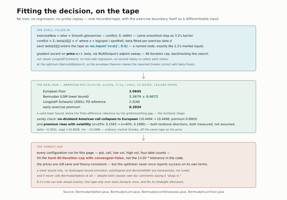
BermudanLsm doesn't call BermudanOption at all — despite both classes'
own doc comments describing it as something that "plugs in" to the
shell's Phase-3 hook, it's a separate implementation of the same
schedule with one difference: the continuation value at each date is a
degree-polyDegree polynomial in log-moneyness, x = log(spot / spotRef),
whose coefficients are named tape inputs:
ADouble x = s.div(sRef).log();
ADouble contEst = rec.constant(0.0);
ADouble xp = rec.constant(1.0);
for (int j = 0; j < perDate; j++) {
  contEst = contEst.add(rec.input("cv:" + d + ":" + j, 0.0).mul(xp));
  xp = xp.mul(x);
}
That rec.input("cv:d:j", ...) is the exact same mechanism 2.2 found
behind every market Greek — a named INPUT node whose gradient you can
read back by name. Here it isn't market data; it's an optimization
variable. BermudanLsm.price runs a backtracking gradient ascent, up to
40 iterations, pushing every beta[d][j] in the direction that increases
price, using MultiOutput's adjoint gradient at each step — one forward
sweep, one reverse sweep, no finite differences anywhere in the loop.
The class is named BermudanLsm and its own doc comment calls it
"least-squares Monte-Carlo," but it is not the textbook Longstaff-Schwartz
(2001) algorithm. Classic LSM replays each path once to collect
in-the-money states, fits a cross-sectional regression on the host, then
replays again with the fitted continuation plugged in. This does none of
that: beta is optimized by gradient ascent on price, directly on the
tape, with no separate regression step and no second replay. Because a
sub-optimal exercise policy can only ever lose value, the optimized price
is still a valid lower bound on the true American price — and because
d(price)/d(beta) = 0 at the optimum, the envelope theorem says the
market Greeks read off the same tape with beta held fixed are correct to
first order, with no need to differentiate through the fitting loop at
all.
The real run
BermudanLsmShowcase prices an American put at Longstaff-Schwartz's own
Table 1 parameters (S=K=40, σ=20%, T=1y, r=6%), 25 exercise dates,
150,000 paths, seed 42:
| price | |
|---|---|
| European floor | 2.0645 |
| Bermudan (LSM lower bound) | 2.2679 ± 0.0072 |
| Longstaff-Schwartz (2001), finite difference | 2.3140 |
The early-exercise premium is 0.2034 — below the finite-difference
reference by 0.046, which is exactly the shape a lower bound should
have: a smoothed, polynomial-fitted policy is never quite as good as the
finite-difference method's near-exact boundary, so the price sits a
little under it, never over. The same reverse sweep that produced the
price also hands back delta −0.3932, vega +14.8658, and rho
−12.0486 — ordinary market Greeks, with beta frozen at its optimized
value per the envelope-theorem argument above.
Two sanity checks confirm the optimizer is finding something real, not
just a number near the reference by luck. An American call on a
non-dividend stock (S=K=100, σ=20%, r=5%) should never exercise
early — textbook result, no dividend to capture by exercising before
expiry — and the optimized policy finds exactly that: European 10.4494
against Bermudan 10.4498, a premium of 0.0003, indistinguishable from
Monte-Carlo noise. And raising volatility on the put from 20% to 40%
raises the early-exercise premium from 0.1583 to 0.1990, the direction
theory predicts, both numbers from real runs at matched dates, paths, and
seed.
Try it yourself
Holding the market and every other parameter fixed and varying only the number of exercise dates on the put above:
| exercise dates | early-exercise premium |
|---|---|
| 5 | 0.1155 |
| 10 | 0.1624 |
| 25 | ? |
More exercise opportunities should push the Bermudan premium up, toward
the continuous-exercise American limit — predict roughly where 25
lands before you run it. (It keeps climbing, but the jump from 10 to
25 is smaller than the jump from 5 to 10: you're approaching a
limit, not climbing a straight line.)
▶️ Run it
mvn -o -q -pl nablatensor-examples exec:java \
  -Dexec.mainClass=com.nablatensor.examples.BermudanLsmShowcase -Dpaths=150000 -Ddates=25
cpu-jit implicitly — MultiOutput.of(...).on("cpu-jit") is hardcoded
inside BermudanLsm.price, so there's no engine string to pass here at
all.
⚠️ What this doesn't do
Every configuration run for this page — the put, the call, both
volatilities, all four date counts in the table above — hit the
hard-coded 40-iteration cap with converged=false, never the code's own
1×10⁻⁹ gradient-norm tolerance. The prices are consistently sane and
theory-consistent, but the optimizer itself never once reports success by
its own stopping rule; whatever's left on the table past iteration 40 is
unmeasured. This is also a lower bound only — no dual or upper-bound
estimator (the kind that would let you quote a confidence interval that
brackets the true American price from both sides) — and polyDegree and
decisionWidth are parameters you choose, not ones the fit picks for
you. It prices vanilla puts and calls on a single GBM underlying with no
dividend; nothing here touches a Bermudan swaption, a multi-asset
early-exercise payoff, or a schedule with unequally spaced dates.
What's next
→ Deeper: American / Bermudan options by least-squares Monte-Carlo has the full pinned-test tolerances this page's sanity checks are drawn from. → Next: Fitting a smile: SABR in two seconds — Module 7 opens with calibration, where the thing being optimized on the tape is a model's own parameters instead of an exercise boundary.