A JIT inside a JIT: how cpu-jit compiles adjoint Greeks into bytecode

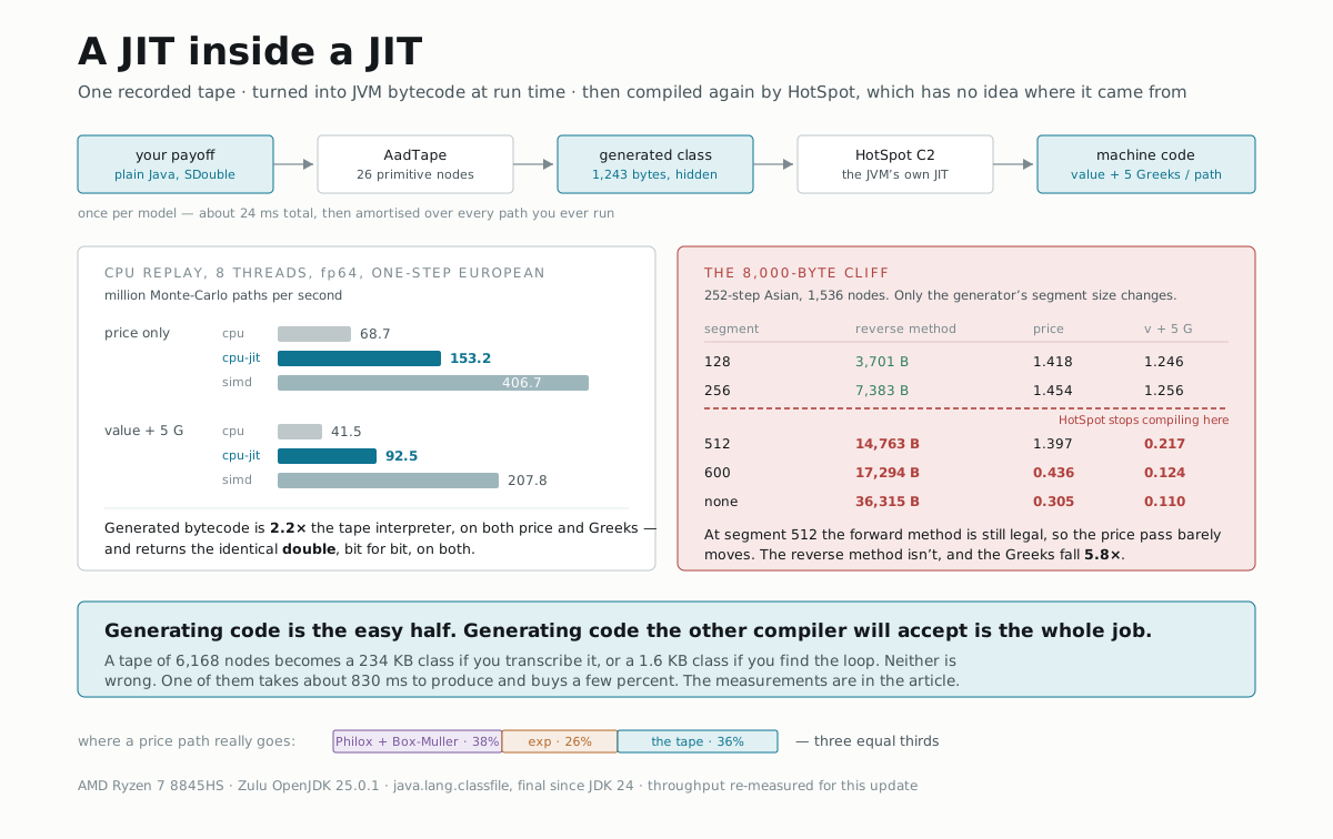
Here is the experiment that made this article worth writing.

Take one recorded Monte-Carlo tape. Compile it to bytecode. Run it. Now change a single number in the code generator — not the maths, not the payoff, not the JVM flags, not the thread count. Just how many tape nodes the generator puts into each emitted method. From 256 to 512.

The price pass barely moves: 1.454 million paths per second before, 1.397 after. The Greeks fall from 1.256 to 0.217. A 5.8× collapse, from a constant that nobody chose deliberately and that does not appear anywhere in the arithmetic.

That is the whole subject of this article in one result. Generating machine code from a tape is the easy half. Generating code that the other compiler — the one already inside your JVM — is willing to look at is the entire job, and the failure mode is not a warning or an exception. It is silence, and a number six times smaller than it should be.

So: what a recorded tape actually is, what cpu-jit turns it into, what those instructions look like one at a time, where the 8,000-byte cliff comes from, why the same class file is 234 KB or 1.6 KB depending on a flag, and — the part that reframes everything else — what fraction of a Monte-Carlo path the compiled tape is responsible for at all.

Every throughput number below was re-measured on referential machine (Ryzen 7 8845HS, 8 cores, Zulu OpenJDK 25.0.1) for this update, except the single-threaded cost breakdown in Part eight, which is carried over from the original pass on the same machine and noted where it appears.

Part one: what a tape is

Adjoint algorithmic differentiation rests on a trick that sounds like cheating the first time you meet it and then never stops being useful. You want the derivative of a valuation with respect to a lot of inputs. Instead of differentiating the program, you record what the program did — the actual sequence of arithmetic operations it performed on this particular set of inputs — and then differentiate that.

The recording is called a tape. In NablaTensor it is produced by running your payoff exactly once against a scalar type that computes nothing:

public final class ADouble {
  public ADouble mul(ADouble other) {
    return binary(AadOp.MUL, other);      // appends a node; returns a handle
  }
  public ADouble exp() {
    return unary(AadOp.EXP);
  }
  // ...
}

Every arithmetic method on ADouble appends one entry to the recorder's tape and hands back a reference to that entry. No number is ever computed while recording. By the time your payoff has run once, the tape holds a flat, numbered list: for each node, an opcode, up to two argument indices, and possibly a constant.

That is the entire intermediate representation. Here is a real one — the complete tape for a one-step European call, printed straight out of the engine:

european steps=1 nodes=26 inputs=5 randTotal=1 output=25
  0  INPUT  v0   = in[0]  // spot                active
  1  INPUT  v1   = in[1]  // strike              active
  2  INPUT  v2   = in[2]  // vol                 active
  3  INPUT  v3   = in[3]  // rate                active
  4  INPUT  v4   = in[4]  // maturity            active
  5  MUL    v5   = v2 * v2                       active
  6  CONST  v6   = 0.5                           -
  7  MUL    v7   = v5 * v6                       active
  8  SUB    v8   = v3 - v7                       active
  9  CONST  v9   = 1.0                           -
 10  MUL    v10  = v4 * v9                       active
 11  MUL    v11  = v8 * v10                      active
 12  SQRT   v12  = sqrt(v10)                     active
 13  MUL    v13  = v2 * v12                      active
 14  RANDN  v14  = randn #0                      -
 15  MUL    v15  = v13 * v14                     active
 16  ADD    v16  = v11 + v15                     active
 17  EXP    v17  = exp(v16)                      active
 18  MUL    v18  = v0 * v17                      active
 19  SUB    v19  = v18 - v1                      active
 20  CONST  v20  = 0.0                           -
 21  MAX    v21  = max(v19, v20)                 active
 22  NEG    v22  = -v3                           active
 23  MUL    v23  = v22 * v4                      active
 24  EXP    v24  = exp(v23)                      active
 25  MUL    v25  = v21 * v24                     active

Read it and the whole Black-Scholes path falls out. Nodes 5–8 build r − σ²/2. Node 10 is T × 1.0 (the time grid's fraction of maturity for a one-step grid). Node 11 is the drift over the step; nodes 12–15 the diffusion σ√T·Z; node 17 the exponential; node 18 the terminal spot. Nodes 19–21 are max(S(T) − K, 0), and 22–25 discount it. Twenty-six operations, five of which are the inputs you want Greeks for.

There is no if, no loop, no function call, no object. That is not a limitation of the recorder — it is the point. A tape is a straight-line program over scalars, and a straight-line program over scalars is the easiest thing in the world to compile, to vectorise, to ship to a GPU, or to walk backwards.

The two schools, and the third thing

By the 1990s the AD community had settled into two camps, and the split is worth understanding because cpu-jit sits in neither.

Source transformation reads your Fortran or C at build time and writes new source that computes the derivative — ADIFOR, Tapenade, TAF. The output is ordinary code, compiled by your ordinary compiler, and it is fast, because the optimiser sees everything. It is also rigid: your program has to be the kind of thing the transformer can parse and reason about, and you re-run the tool every time you change a line.

Operator overloading — ADOL-C, CppAD, NAG's dco/c++, and NablaTensor's ADouble — replaces double with an active type that records as it goes. It handles anything the host language can express, including branches and library calls, because it only ever sees what actually executed. The cost is that somebody has to run the tape afterwards, and running a tape is interpretation.

cpu-jit is a third thing: overload to record, then transform to source at run time. The recording is as flexible as overloading, because it is overloading. The execution is as fast as source transformation, because by the time paths are running the tape has been turned into instructions. What makes it possible is that the JVM will happily accept a class you invented ten milliseconds ago.

Part two: why not just interpret it?

You have a tape. The obvious thing to do with it is walk it. NablaTensor's cpu engine does exactly that, and its inner loop is about as tight as a tape interpreter gets:

for (int i = 0; i < n; i++) {
  int a = argA[i];
  int b = argB[i];
  v[i] = switch (ops[i]) {
    case CONST -> constants[i];
    case INPUT -> in[a];
    case RANDN -> rng[b].normal();
    case ADD   -> v[a] + v[b];
    case MUL   -> v[a] * v[b];
    case EXP   -> Math.exp(v[a]);
    // ...nine more
  };
}

The arrays are flattened once in the constructor, so there is no virtual call per node and no pointer chasing. This is a good interpreter. And it is still doing, for every one of the 26 nodes, on every one of a hundred million paths: three array loads with bounds checks (argA[i], argB[i], ops[i]), a tableswitch on the opcode, and an indirect branch that the hardware branch predictor has no hope of getting right, because the op sequence is MUL, CONST, MUL, SUB, CONST, MUL, MUL, SQRT, … and predictors are trained on repetition, not on a specific 26-long word.

The multiply itself is one instruction. Everything around it is bookkeeping to answer a question — which operation is this? — that was already settled before the first path ran.

Measured on referential machine, eight threads, fp64, the one-step European:

engine	threads	price only	value + 5 Greeks	adjoint cost
cpu (tape interpreter)	1	11.5 Mpath/s	6.8 Mpath/s	1.69×
cpu-jit (generated bytecode)	1	22.8	14.7	1.55×
cpu	8	68.7	41.5	1.66×
cpu-jit	8	153.2	92.5	1.66×
simd (JDK Vector API)	8	406.7	207.8	1.96×

Two things to read off. The generated kernel is a straight 2.2× over a good interpreter, on both price and Greeks — that is the cost of dispatch, and nothing else, because the two engines execute the identical sequence of floating-point operations. And the adjoint sweep costs about 1.66× a price pass, not the 11× a five-Greek central-bump ladder would cost. That is the whole argument for adjoint AD, and it is orthogonal to everything in this article: it holds on the interpreter too.

Part three: emitting the code

Now the interesting part. How do you turn that tape into a class?

Until recently the answer on the JVM was "use ASM", the bytecode library that has quietly underpinned Spring, Hibernate, Kotlin, Mockito and roughly everything else since 2002. Since JDK 24 there is a standard answer in the platform: java.lang.classfile, the Class-File API.

The generator is a walk over the tape with one case per opcode. This is the entire forward emitter, with only two debug probes elided:

private static void fwdNode(CodeBuilder cb, Tape tp, int i, Slots s, T t) {
  int a = tp.a[i], b = tp.b[i];
  switch (tp.op[i]) {
    case CONST -> s.storeV(cb, i, () -> t.load(cb, tp.k[i]));
    case INPUT -> s.storeV(cb, i, () -> s.loadInput(cb, a));
    case RANDN -> s.storeV(cb, i, () -> s.loadDraw(cb, i));
    case ADD   -> s.storeV(cb, i, () -> { s.loadV(cb, a); s.loadV(cb, b); t.add(cb); });
    case MUL   -> s.storeV(cb, i, () -> { s.loadV(cb, a); s.loadV(cb, b); t.mul(cb); });
    case EXP   -> s.storeV(cb, i, () -> { s.loadV(cb, a); t.math1(cb, "exp"); });
    case MAX   -> s.storeV(cb, i, () -> { s.loadV(cb, a); s.loadV(cb, b);
                                          cb.invokestatic(CD_MATH, "max", t.mathBin()); });
    // ...
  }
}

storeV and loadV are an interface, not a fixed emission — that indirection is what lets the same fifteen formulas serve the flat kernel (values in an array) and the rolled kernel (values in JVM locals) without a second copy of the derivative rules. It matters later.

Here is what comes out. This is javap -c on the class the engine actually generated for the tape above, at node 18 — v18 = v0 × v17:

168: aload_0                     // the v[] array
169: bipush        18            // the destination slot — a literal
171: aload_0
172: iconst_0                    // node 0's slot — a literal
173: daload                      // v[0], the spot
174: aload_0
175: bipush        17            // node 17's slot — a literal
177: daload                      // v[17], exp(drift + vol*Z)
178: dmul
179: dastore                     // v[18] = the product

Ten instructions, and every index that the interpreter would have had to fetch out of a parallel array is a constant sitting in the instruction stream. The JVM has no registers at the bytecode level, so values move through an operand stack: push, push, consume-two-push-one.

Where the class goes

The bytes come back as a byte[], and then:

Class<?> cls = MethodHandles.lookup().defineHiddenClass(bytes, true).lookupClass();
return cls.getConstructor().newInstance();

A hidden class — JEP 371, JDK 15. It has no binary name that any class loader will resolve, so nothing can link against it, reflect it by name, or accidentally hold it alive. It is unloadable independently of its loader, so closing a pricer really does let the kernel go. And it is not an exotic corner of the JVM: it is the mechanism invokedynamic uses for lambdas, which means your JVM has been generating and loading hidden classes since long before you asked it to generate one on purpose. Hidden classes replaced sun.misc.Unsafe.defineAnonymousClass, which did the same job for years while being, by name and by nature, something nobody was supposed to be using.

The generated class implements a two-method interface:

public interface JitKernel {
  double forward(double[] v, double[] in, double[] draws, double[] scratch);
  void   reverse(double[] v, double[] d, double[] scratch, double[] draws);
}

Which means the replay loop — the part that runs a hundred million times — is two megamorphic-free virtual calls into straight-line code:

kernel64.forward(v, in, draws, scratch);
acc.value += v[outputNode];
if (adjoints) {
  Arrays.fill(d, 0.0);
  d[outputNode] = 1.0;
  kernel64.reverse(v, d, scratch, draws);
  for (int j = 0; j < grad.length; j++) grad[j] += d[inputNode[j]];
}

d[outputNode] = 1.0 is the entire seeding ritual of reverse-mode AD: the derivative of the output with respect to itself. Everything else is the tape propagating it.

Part four: the reverse sweep is code too

The forward sweep is a transcription. The reverse sweep is where the code generator earns its name, because there is no source program to transcribe — the adjoint of a tape is something you derive, one local rule per opcode:

case MUL -> {
  s.addD(cb, a, () -> { s.loadD(cb, i); s.loadV(cb, b); t.mul(cb); });   // d[a] += d[i] * v[b]
  s.addD(cb, b, () -> { s.loadD(cb, i); s.loadV(cb, a); t.mul(cb); });   // d[b] += d[i] * v[a]
}
case EXP  -> s.addD(cb, a, () -> { s.loadD(cb, i); s.loadV(cb, i); t.mul(cb); });
case LOG  -> s.addD(cb, a, () -> { s.loadD(cb, i); s.loadV(cb, a); t.div(cb); });
case SQRT -> s.addD(cb, a, () -> { s.loadD(cb, i); t.load(cb, 0.5); t.mul(cb);
                                   s.loadV(cb, i); t.div(cb); });

Three of these are worth pausing on.

EXP reads v[i] — its own forward output — rather than recomputing exp(v[a]). Because d/dx e^x = e^x, and the forward sweep already left the answer in v[i]. The same trick works for SQRT. This is why keeping the forward values around is not a memory tax you tolerate; it is the thing that makes the reverse sweep cheap.

MAX has no derivative at the kink, so the generator emits a branch:

 96: dcmpg                       // compare v[19] and v[20]
 98: iflt          115
101: ... d[19] += d[21]          // the option is in the money
112: goto          126
115: ... d[20] += d[21]          // it is not; the adjoint dies here

Which is exactly the right answer for a payoff: on paths that finish out of the money, the whole sensitivity chain terminates at node 21 and never reaches the inputs. The kink is measure-zero and the estimator is unbiased, and the branch is what makes it so.

And every rule is +=, never =, because a node may be read by several later nodes and its adjoint is the sum of the contributions. Node 2 (vol) is read at node 5 twice and again at node 13 — three contributions. In bytecode a read-modify-write on an array element wants the array reference and index on the stack twice, so the generator uses dup2:

148: aload_1                     // the d[] array
149: iconst_0                    // slot 0
150: dup2                        // duplicate both — one pair to read, one to write
151: daload                      // d[0]
... compute the contribution ...
161: dadd
162: dastore                     // d[0] = d[0] + contribution

The consequence for code size is what sets up the next section. Look back at the tape figure: INPUT, CONST and RANDN rows emit nothing in reverse, but every MUL emits two full read-modify-write accumulations. Measured on the real generated classes, the reverse sweep for a given block of nodes is about 2.5× the bytecode of the forward sweep for the same block.

Part five: the 8,000-byte cliff

Here is the trap.

A straight-line transcription of an n-node tape produces roughly 11 bytes of forward bytecode and 29 bytes of reverse bytecode per node. For the 26-node European that is a 1,243-byte class and nobody cares. For a 252-step Asian — 1,536 nodes — the forward sweep alone would be about 20 KB of bytecode in a single method.

HotSpot will not compile that method. Ever.

The relevant flag is -XX:+DontCompileHugeMethods, on by default, and its threshold HugeMethodLimit, 8,000 bytes of bytecode. (It is a HotSpot develop flag, so it does not show up in -XX:+PrintFlagsFinal on a production build — but the measurements below bracket it between 6,836 and 8,067, which is about as close as you can get to reading a constant out of a black box.) A method over that size is skipped by the JIT compiler entirely and executes in the bytecode interpreter for the life of the process. There is no warning. Nothing throws. Your carefully generated kernel simply runs at interpreter speed, which is worse than the tape interpreter you were trying to beat, because at least that one gets compiled.

So KernelGenerator splits both sweeps into fwd$0, fwd$1, … and rev$0, rev$1, … of at most segNodes nodes each — 128 by default — and the public forward/reverse methods are nothing but a list of invokestatic calls. Values that cross a segment boundary live in the shared v[]/d[] arrays, which they were living in anyway.

To find out what that is worth, I varied the segment size on the 1,536-node Asian and measured both the emitted method sizes and the throughput:

-Dnablatensor.jit.seg	fwd$k bytes	rev$k bytes	price	value + 5 Greeks
128 (default)	1,463	3,701	1.418 Mpath/s	1.246 Mpath/s
256	3,249	7,383	1.454	1.256
512	6,836	14,763	1.397	0.217
600	8,067	17,294	0.436	0.124
(off — one method each)	21,286	36,315	0.305	0.110

The seg = 512 row is the one to stare at. The forward method is 6,836 bytes — under the limit, compiled, fine — and the price pass is essentially unaffected: 1.397 against the default's 1.418. The reverse method is 14,763 bytes, over the limit, never compiled, and the adjoint pass falls 5.8×. One tuning constant selectively destroyed the Greeks and left the price alone, because the forward/reverse bytecode ratio put the two sweeps on opposite sides of an 8,000-byte line.

Push to seg = 600 and the forward method crosses too, at 8,067 bytes, and now the price pass collapses as well.

The general lesson is one every code generator learns eventually and this one learned the expensive way. When you generate code, you are not writing to a machine. You are writing to another compiler, and that compiler has opinions, budgets and cliffs. MaxInlineSize is 35 bytes. FreqInlineSize is 325. HugeMethodLimit is 8,000. None of those numbers are in your problem domain, and all of them are in your performance profile.

Part six: unrolled by default, rolled on request

The flat kernel is a full unroll. A 252-step Asian becomes 1,536 nodes becomes a 59 KB class; a 1,024-step tape becomes 6,168 nodes and a 234 KB class. That is a lot of instruction cache for a loop body you wrote once.

So there is a second code generator. JitOptimizations.Level.LOW_RISK turns on loop detection: scan the tape for a prologue · body×N · epilogue shape, confirm that every block is structurally identical up to a constant index shift, and emit the body once inside a real bytecode loop. Values that live across an iteration become JVM locals instead of array slots; the values the reverse sweep needs per iteration go into a compact step tape.

That last part is checkpointing, and it is the subtle bit. A rolled forward loop overwrites its locals every iteration, but the reverse sweep needs each iteration's values. So the generator works out exactly which body positions the adjoint rules read — MUL needs both arguments, EXP needs only its own output, ADD needs nothing — and tapes only those, iters deep. For the Asian that is two values per step out of a six-node body. The detector reports its findings honestly if you ask it:

[jit] rolled(period=6 x251, tape=2) nodes=1536 fp64 classBytes=1664

Six-node body, 251 iterations, two values taped per iteration. The class went from 59,176 bytes to 1,664.

And now the honest part, which is not what the project's own internal notes said.

Where it would pay: tapes far larger than instruction cache, or a process that builds thousands of pricers where 234 KB of class metadata each starts to add up. Neither is the 26-node European.

One footnote on those generation times, because it is the same joke one level up: the ~20 ms quoted earlier for building the European kernel is the first one in the process. The second model built in the same JVM takes about 1.6 ms, because by then HotSpot has compiled the code generator. The compiler that compiles your payoff needed compiling too.

Part seven: does it compute the same number?

A code generator that is fast and subtly different is worse than no code generator, because you will find out about the difference from a P&L attribution meeting.

So: same tape, same seed, same path count, every CPU replay strategy this engine has, printed to seventeen significant digits.

european steps=1 paths=2,000,000 seed=42
engine   thr  jit        price                  delta                  vega
cpu      1    -          9.4094807415033050     0.59872260307813430    38.644884800242730
cpu      8    -          9.4094807415028880     0.59872260307811660    38.644884800241820
cpu-jit  1    -          9.4094807415033050     0.59872260307813430    38.644884800242730
cpu-jit  8    -          9.4094807415028880     0.59872260307811660    38.644884800241820
cpu-jit  8    LOW_RISK   9.4094807415028880     0.59872260307811660    38.644884800241820
simd     8    -          9.4094807415028900     0.59872260307811790    38.644884800241720
analytic -    -          9.4133976292812000     0.59870630802372290    38.666811680284930

The interpreter and the generated kernel agree bit for bit — at one thread, at eight threads, and with the rolled generator on. Not "to seven figures"; identically, all 53 bits of mantissa.

That is not luck, it is a design constraint. The default code generator emits Math.exp, not a faster polynomial; it emits a*b in the recorded order rather than reassociating; it accumulates adjoints in tape order. Every one of those is a place where a couple of percent was available and was left on the table so that the answer would not move. If you want the percent, you name the optimisation and accept that the low bits change — FAST_MATH says so in its own Javadoc.

The 1-thread and 8-thread rows do differ, in the sixteenth digit. That is summation order across workers: eight partial sums added in a different sequence than one running total. It is inherent to parallel reduction, it is about 4×10⁻¹⁶ relative, and Monte-Carlo standard error on two million paths is around 10⁻²·⁵. The physics of the estimator dwarfs it by thirteen orders of magnitude.

On the 1,536-node Asian the picture is very slightly looser: at eight threads cpu, flat cpu-jit and rolled cpu-jit are still bit-identical (5.3106693425412870), while at one thread the generated kernels differ from the interpreter in the last digit (…413450 versus …413460). Longer tape, more places for C2 to contract a local += x*y into a fused multiply-add in one shape and not the other. One ULP, documented, on a 200,000-path estimate whose own standard error is in the third decimal.

Part eight: what is actually expensive

(The breakdown in this section is carried over from the original pass rather than re-measured for this update — it is a single-threaded, isolated-microbenchmark methodology that is sensitive enough to machine load that a stale, carefully-built number is more trustworthy than a rushed fresh one. Everything else in this article was re-measured.)

Now the section that puts everything above in perspective — and that I had to measure twice, because the obvious way to measure it is wrong.

The engine carries two probes for exactly this question: -Dnablatensor.jit.randn=zero, which emits a literal 0.0 for every draw instead of reading the RNG buffer, and -Dnablatensor.jit.exp=none, which emits the identity for EXP. Both produce deliberately wrong prices. Both are meant to answer "what would this cost if that part were free?"

One of them does not answer it. Zeroing the draw does not only remove the RNG. With Z a literal zero, vol × Z folds away, the whole log-return drift + vol·Z becomes loop-invariant, and C2 hoists exp(·) clean out of the path loop with it. The probe deletes the generator and both transcendentals, then hands the entire saving to the generator. It reports a number that is almost twice the truth.

So here is the breakdown again, measured with levers that do not fold, and at one thread so there is no turbo or memory-contention confound. One-step European, fp64, price pass:

component	ns/path	share	how it was measured
Philox + Box-Muller	15.9	38%	the engine's own generator code lifted verbatim into a standalone loop in the same call shape, 40 M draws, best of 11
the two exp calls	11.1	26%	-Dnablatensor.jit.exp=none: 23.6 → 32.0 Mpath/s. The draws stay live, so nothing folds
the tape, plus accumulation	15.4	36%	the residual
one price path	42.3		23.6 Mpath/s
the reverse sweep on top	26.3		14.6 Mpath/s for value + five Greeks

Roughly three equal thirds. The random draw is the largest single item at 38%, but it is not the two-thirds the naive probe claimed, and the recorded tape — the thing this entire article is about compiling — is a third of the bill, not a sixth.

One honest test of that attribution: if the draw really is 15.9 ns of a 42.3 ns path, then making the draw 1.74× cheaper should buy about 1.19× on the path. I built that experiment — swapping Box-Muller for an inverse-CDF quantile function, which turns three transcendental calls per draw into one rational polynomial — and measured 1.12× end to end. Close, and short by exactly the amount you would expect: an out-of-order core overlaps part of the draw with the tape, so only about two thirds of any saving on the draw reaches the bottom line. About 65% of it did.

That reframes the exercise without undermining it. The code generator's job was never to make the tape's arithmetic fast — it is the same arithmetic either way. Its job was to make the tape stop costing anything beyond its arithmetic, so that what is left is a third of a path of real floating-point work, a third of a path of transcendentals, and a third of a path of random numbers, all of which you genuinely asked a computer to do.

What to actually use

The full CPU picture on this box, all engines pinned to eight threads for a fair comparison, one fresh JVM per row:

engine	precision	price only	value + 5 Greeks	needs
cpu — tape interpreter	fp64	68.7 Mpath/s	41.5 Mpath/s	nothing
cpu-jit — generated bytecode	fp64	153.2	92.5	JDK 24+
simd — JDK Vector API	fp64	406.7	207.8	--add-modules jdk.incubator.vector

cpu-jit is the default engine, and the reasoning is not that it is the fastest, because it isn't — simd is 2.7× quicker on the price pass. It is the default because of what it doesn't need. No incubator module, no --add-modules on a production command line, no native library, no device driver, no GPU. It runs on a stock LTS JVM in a locked-down container, it is bit-exact against the reference interpreter, and it is twice the interpreter. For a risk system that has to justify every dependency to somebody, that combination is worth more than a factor of two.

Reach past it when you have measured that you need to: simd when the incubator module is acceptable, vulkan or cuda when a laptop iGPU beating both CPU paths by 30× is worth a driver dependency.

And the ranking of things that actually mattered, in order:

1. Not being interpreted at all. 2.2× over a good tape interpreter, for free, from a compiler with no dependencies.
2. Emitting methods HotSpot will compile. Up to 5.8× on the adjoint sweep, and the failure is silent, which makes it the one to get right first.
3. Loop rolling. A few percent on the adjoint sweep of a 252-step tape, noisily, a 144× reduction in class size, and around 830 ms of generation time. Opt-in for a reason.
4. Everything else. FAST_MATH — hand-rolled polynomial log/sin/cos for the Box-Muller step — is documented in its own Javadoc as measuring slower on Zen 4 than the SVML-backed Math intrinsics it replaces, while also moving the low bits. It ships anyway, disabled, so that the result is on the record rather than folklore.

Try it

Everything here is reproducible from the public repo. The tape dump is four lines against the public API:

var model = Nabla.model(EquityMarket.atmOneYear(),
    (rec, in) -> Products.europeanCall().record(rec, in, TimeGrid.uniform(1)));
AadTape t = model.tape();
for (int i = 0; i < t.size(); i++) {
  System.out.println(i + "  " + t.op(i) + "  a=" + t.argA(i) + " b=" + t.argB(i));
}

To watch the generator make its decisions, set -Dnablatensor.jit.debug=1 and it prints the shape, node count, precision and emitted class size for every kernel it builds. To reproduce the cliff, set -Dnablatensor.jit.seg and walk it upward on a tape of a few hundred nodes; the collapse arrives between 256 and 512 on this payoff and will arrive somewhere else on yours, because where it arrives depends on how much bytecode your adjoint rules emit per node.

Which is, in the end, the moral. The number that governs whether your generated Greeks run at full speed or an order of magnitude below it — the widest gap measured here was 1.256 against 0.110 Mpath/s, a factor of more than eleven — is not in your model, your market data or your maths. It is a bytecode budget in somebody else's compiler, and the only way to find out where you stand against it is to measure.

Source: KernelGenerator.java (the code generator), JitReplay.java (the replay loop), ScalarReplay.java (the interpreter it is measured against) and JitOptimizations.java (what is opt-in and why).