Bump-and-revalue is quietly costing you 10x

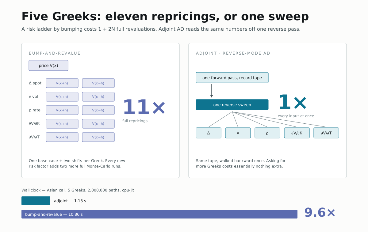
If your Monte-Carlo risk engine reports delta, vega and rho by shifting each input a little and repricing, you already know the drill: five Greeks means at least eleven full revaluations of the book — one base case, plus two shifted prices per Greek for a central difference. Nobody sat down and decided that's the right amount of compute to spend. It's just what falls out of the only tool most engines have: the price.

(V(x+h) - V(x-h)) / 2h — a Greek is a slope, and the price is a single point on that slope, so you buy the slope by evaluating two more points. Do that for every risk factor and the replay count is 1 + 2N. It is simple, it is exact enough, and it is the reason risk runs take longer than pricing runs by a factor that grows with every new Greek someone asks for.

The other way to get a slope

Adjoint algorithmic differentiation doesn't reprice at all. It records the valuation once as a tape of primitive operations, then walks that tape backwards a single time. One reverse sweep reads off the sensitivity to every input simultaneously — not because it's cheating the math, but because the chain rule composes the same way whichever direction you walk it, and walking backwards from one output is cheap regardless of how many inputs there are. The cost is a small constant on top of the price, not a multiple of it.

A payoff expression drawn as a graph twice. Left, 'forward pass': five nodes — inputs S0, sigma, r feeding S(T), then p = max(S(T) - K, 0), then V — each computed and holding a value, arrows pointing up. Right, 'reverse pass': the same graph with one set of arrows pointing down from V, each node now holding the partial derivative of V with respect to itself; the three input nodes are filled in simultaneously and tagged delta, vega, rho. Caption: the reverse pass touches each node once, so its cost is flat in the number of inputs while bump-and-revalue's grows as 1 + 2N. — The forward pass records each node once. The reverse pass then walks the same edges once, in the opposite direction, and every input’s sensitivity falls out of that single traversal — adding a fourth or fortieth input doesn’t lengthen the walk.

In NablaTensor that's the difference between two method calls:

MonteCarlo<EquityMarket> adjoint = MonteCarlo.of(Products.asianCall())
    .market(market).steps(steps).greeks().on(engine).build();       // value + all Greeks

MonteCarlo<EquityMarket> priceOnly = MonteCarlo.of(Products.asianCall())
    .market(market).steps(steps).priceOnly().on(engine).build();    // value alone

.greeks() compiles a kernel that does the forward pass and the reverse sweep. .priceOnly() compiles a kernel that only does the forward pass. Everything else about the recording — the payoff, the model, the number of scenarios — is identical. The only thing that changes is whether you throw away the tape or walk it back.

Reading the numbers back out is where the asymmetry shows. The adjoint kernel runs once, and every sensitivity is already sitting on the result — one accessor per input, each naming a node the reverse sweep already walked to:

var v = adjoint.run(scenarios, seed);

double price = v.price();
double delta = v.greek(EquityMarket::spot);   // dV/dS0
double vega  = v.greek(EquityMarket::vol);    // dV/dsigma
double rho   = v.greek(EquityMarket::rate);   // dV/dr
// ...add EquityMarket::strike, ::maturity — still the same one run.

Bump has no such object to read from. Each Greek is a fresh pair of runs at a shifted market, and the "accessor" is a finite difference:

double h = 1e-4 * market.spot();
double delta =
    (priceOnly.run(market.withSpot(market.spot() + h), scenarios, seed).price()
   - priceOnly.run(market.withSpot(market.spot() - h), scenarios, seed).price()) / (2 * h);
// vega repeats it around market.withVol(...), rho around market.withRate(...), and so on.

Nobody hand-writes the bump loop either — MonteCarlo.of(...).priceOnly() run 1 + 2N times at shifted markets is the bump-and-revalue implementation here. Same builder, same engine, same seed. The comparison below isn't adjoint-tuned-code versus a naive competitor; it's the same code path measured two ways.

The number, reproduced live

We didn't want to just repeat the number from the repository's own docs, so we reran the benchmark on the machine this article was written on, right before publishing it:

$ mvn -o -q install
$ mvn -o -q -pl nablatensor-bench exec:java \
    -Dexec.mainClass=com.nablatensor.bench.Benchmarks -Dscenarios=2000000 -Dsteps=252

# NablaTensor benchmark

- machine   : JDK 25.0.1+8-LTS, Linux amd64, 16 processors
- product   : Asian call, 252 fixings, fp64
- scenarios : 2,000,000   seed : 42

## adjoint vs bump-and-revalue  (engine cpu-jit)

| method | replays | wall clock | speedup |
|---|--:|--:|--:|
| adjoint (value + 5 Greeks, one sweep) | 1 | 1.1259 s | 9.6x |
| central bump (1 + 2x5 price-only) | 11 | 10.8633 s | 1.0x |

adjoint: price=5.301676 delta=0.561932 vega=22.389375 rho=23.603735

Both rows compute the same five numbers — price, delta, dV/dK, vega, rho, dV/dT — from the same tape at the same seed. One took 1.13 seconds. The other took 10.86 seconds to arrive at numbers that agree with the first to six decimal places. That's not a rounding-friendly cherry-pick: it's every run of this benchmark, because both paths share the exact same kernel-generation code and differ only in whether the reverse sweep runs once or not at all.

It's not just the Asian call

A single flattering product would be a weak argument, so the repository ships a second harness that runs the same comparison across eight different payoffs — vanilla, path-dependent, barrier, and the kind of exotic structures that show up on real books. We reran that one too:

$ mvn -o -q -pl nablatensor-bench exec:java \
    -Dexec.mainClass=com.nablatensor.bench.ProductBench -Dscenarios=1000000 -Dsteps=128

# Per-product: adjoint vs bump  (engine cpu-jit, 1,000,000 scenarios, 128 steps, seed 42)

| product | price | delta | adjoint | bump (1+2x5) | speedup |
|---|--:|--:|--:|--:|--:|
| European call | 9.41940 | 0.59945 | 0.2853 s | 2.7477 s | 9.6x |
| Asian call | 5.31633 | 0.56212 | 0.2856 s | 2.6971 s | 9.4x |
| Lookback call | 17.12529 | 1.14170 | 0.3182 s | 2.7610 s | 8.7x |
| Floating lookback | 15.46483 | 0.15465 | 0.3156 s | 2.8239 s | 8.9x |
| Barrier up-and-out | 3.22952 | 0.05093 | 0.4876 s | 3.9205 s | 8.0x |
| Digital cash-or-nothing | 0.50541 | 0.01926 | 0.2773 s | 2.6671 s | 9.6x |
| Cliquet | 8.97174 | -0.00000 | 0.4198 s | 3.2269 s | 7.7x |
| Autocallable | 97.86984 | 0.05746 | 0.3047 s | 2.7472 s | 9.0x |

Eight products, eight speedups clustered around 8–10x. None of them were picked to make the number look good — that's the whole table the harness prints. The barrier, digital, cliquet and autocallable rows matter for a different reason too: those payoffs have a genuine kink or jump in them, and a raw discontinuous payoff has an adjoint delta that's either undefined or zero almost everywhere. NablaTensor smooths the indicator function under the hood for exactly these products so the adjoint Greek is usable at all — without that, a barrier's "delta" from AD alone would be noise, and bump would win by default. It's the one case in this table where adjoint isn't just faster; it's the only method that gets you an answer worth trusting on the first try.

The same story on a different backend

Everything above ran on cpu-jit — a generated bytecode kernel, still plain JVM. Swap one flag and the identical recording replays on simd, the JDK Vector API backend, no re-record and no code change:

$ mvn -o -q -pl nablatensor-bench exec:java \
    -Dexec.mainClass=com.nablatensor.bench.ProductBench \
    -Dengine=simd -Dscenarios=1000000 -Dsteps=128

# Per-product: adjoint vs bump  (engine simd, 1,000,000 scenarios, 128 steps, seed 42)

| product | price | delta | adjoint | bump (1+2x5) | speedup |
|---|--:|--:|--:|--:|--:|
| European call | 9.41940 | 0.59945 | 0.1281 s | 0.9619 s | 7.5x |
| Asian call | 5.31633 | 0.56212 | 0.1237 s | 0.9678 s | 7.8x |
| Lookback call | 17.12529 | 1.14170 | 0.1356 s | 1.0047 s | 7.4x |
| Floating lookback | 15.46483 | 0.15465 | 0.1232 s | 0.9719 s | 7.9x |
| Barrier up-and-out | 3.22952 | 0.05093 | 0.2554 s | 1.6117 s | 6.3x |
| Digital cash-or-nothing | 0.50541 | 0.01926 | 0.1171 s | 0.9554 s | 8.2x |
| Cliquet | 8.97174 | -0.00000 | 0.1982 s | 1.3510 s | 6.8x |
| Autocallable | 97.86984 | 0.05746 | 0.1262 s | 1.0220 s | 8.1x |

Two things worth noticing. First, every price and delta is identical to the cpu-jit table above, to the digit — that's the path-for-path reproduction the project holds itself to across backends, not a coincidence. Second, the speedup shrinks a little, to roughly 6–8x instead of 8–10x — because SIMD makes the underlying per-scenario cost cheaper, the reverse sweep's fixed overhead is a slightly larger fraction of a smaller number. Adjoint still wins every single row. A faster backend doesn't change the argument; it just moves both timings down together.

Why the gap only gets worse

The ratio here is (1 + 2N) / (1 + adjoint overhead), and only one of those terms grows with the size of your risk ladder. At N = 5 Greeks it's roughly 11 / 1.15. Ask for a full FRTB-style sensitivity set — twenty, thirty risk factors — and bump-and-revalue is now 41 or 61 full Monte-Carlo runs against the same single reverse sweep. The adjoint side barely moves; the tape doesn't get longer just because you asked for more outputs from it.

That's the actual argument for adjoint AD in a Monte-Carlo pricing library. Not "it's more elegant" — it's that the bump loop's cost is a bill that scales with how much risk you want to see, and the reverse sweep's bill doesn't.

Pick a product and a backend, then drag the risk-ladder size to see it for yourself. Every bar comes from one measured fp32 run per backend — cpu-jit, SIMD and Vulkan on the GPU, all at the same scenario count — with N=5 measured directly and every other N extrapolating only the replay count, 1 + 2N:

adjoint · 1 sweep

0.143s

bump · 11 replays

1.438s

product backend risk factors N 510.1x faster · measured

One measured fp32 run per backend, 500k scenarios / 128 steps. Per-replay cost and reverse-sweep overhead are fixed per product/backend; only the replay count, 1 + 2N, grows with N. On Vulkan the reverse-sweep overhead for branch-heavy payoffs (barrier, cliquet, autocallable) is big enough that adjoint stops winning — GPU divergence on conditional payoff logic costs more than one extra sweep saves.

Bump still wins in two honest cases: a tiny tape with only one or two Greeks (the adjoint overhead isn't amortised over enough outputs to pay for itself), and a genuinely non-differentiable payoff with no smoothing available at all. Neither of those describes a real risk ladder, which is the whole point.

Try it yourself

Everything above is reproducible, not just quotable — clone github.com/nablatensor-dev/nablatensor and run the same commands. mvn -o test is green with no GPU and no native library, so the cpu-jit numbers are what a plain laptop gets, not a cherry-picked machine. The simd row needs one extra JVM flag, since the JDK Vector API is still an incubator module:

MAVEN_OPTS="--add-modules jdk.incubator.vector" \
  mvn -o -q -pl nablatensor-bench exec:java \
    -Dexec.mainClass=com.nablatensor.bench.ProductBench -Dengine=simd