The Asian option

Every payoff so far has needed exactly one thing: the price at expiry. What happens the moment a payoff needs the entire path instead — and what does "the entire path" actually cost, once it's a tape instead of a formula?

The whole story

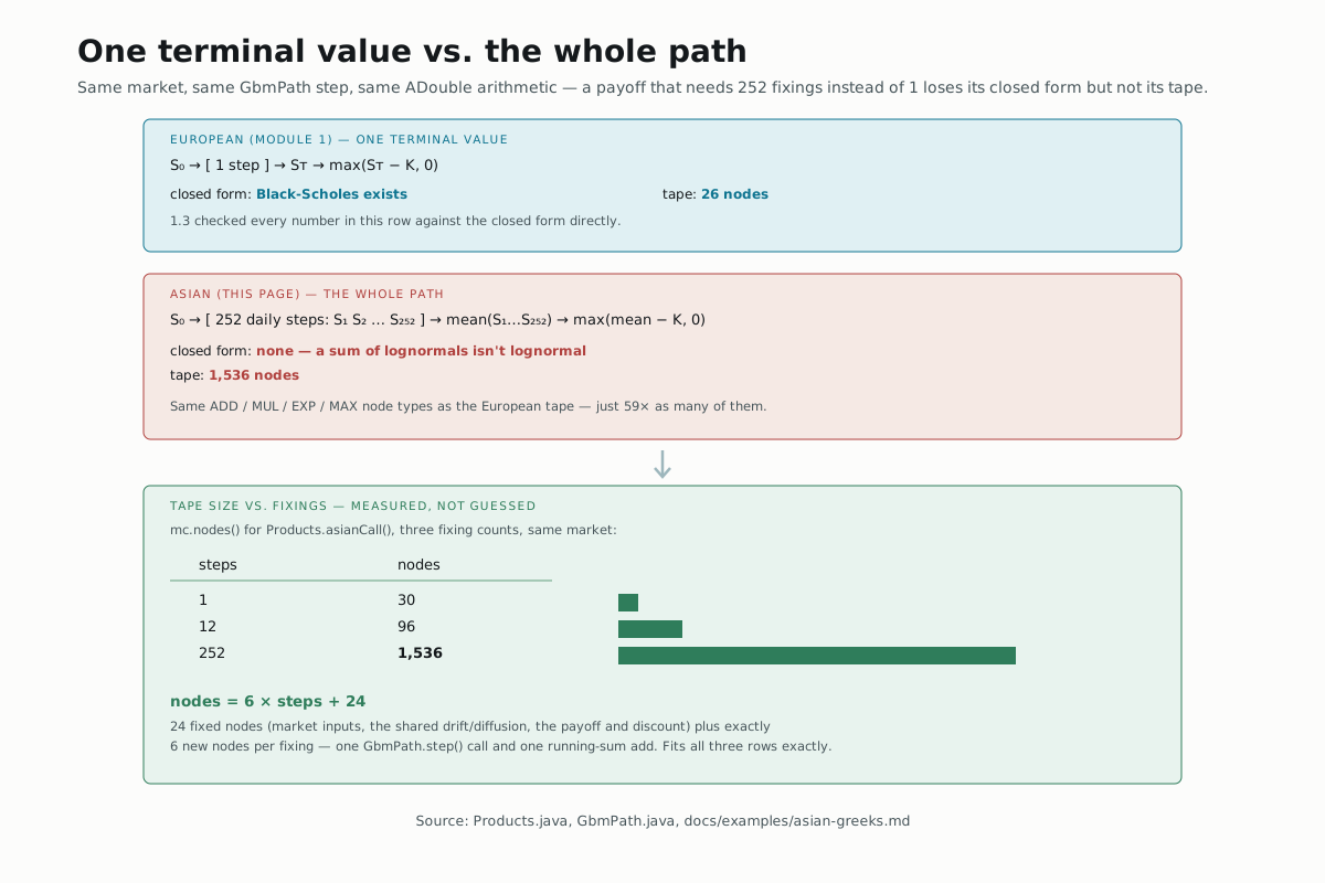
A European payoff needs one terminal value and has a Black-Scholes closed form, recording to a 26-node tape. An Asian payoff averages 252 daily fixings and has no closed form, because a sum of lognormals isn't itself lognormal, recording to a 1,536-node tape. Measuring three fixing counts shows the tape grows by exactly 6 nodes per fixing plus 24 fixed nodes.

Did you know?

An arithmetic-average Asian option has no closed form under GBM, for a reason that's easy to forget once you're used to Black-Scholes: each daily price S_t is lognormal, but their average isn't — a sum of lognormal random variables has no known closed-form distribution. (Their product is lognormal, which is exactly why a geometric-average Asian, unlike this arithmetic one, does have a closed form — a fact quant textbooks lean on constantly and NablaTensor's own docs call out directly.) That's the real reason this payoff needs Monte Carlo: not that nobody has done the algebra, but that the algebra doesn't resolve to anything.

From one step to 252

Products.european and Products.asian are almost the same function — the difference is a loop and a running sum, not a different pricing technique:

public static Product<EquityMarket> asian(OptionType type) {
  return new Named("Asian " + type, (rec, in, grid) -> {
    Sim sim = new Sim(rec, in, grid);
    ADouble path = sim.spot;
    ADouble sum = rec.constant(0.0);
    for (int t = 0; t < grid.steps(); t++) {
      path = sim.model.step(path, rec.randn(), t);
      sum = sum.add(path);
    }
    ADouble average = sum.div((double) grid.steps());
    rec.output(sim.discount(intrinsic(type, average, sim.strike)));
  });
}

Where 1.3's European payoff read sim.spot once and stepped forward once, this one steps forward grid.steps() times — 252, for daily fixings over a year — and accumulates a running sum on every iteration. Same ADouble methods (step's mul/add/exp, intrinsic's sub/max) as Module 1; just called in a loop instead of once.

Did you know?

Each call to sim.model.step(path, rec.randn(), t) records fresh nodes — the spot changes and the random draw is different every time — but the drift and diffusion coefficients it multiplies by don't. GbmPath's own doc comment says why: on a uniform time grid, every step's dt is identical, so the per-step drift and diffusion are each recorded once and the same two ADoubles are reused for all 252 steps, not recomputed 252 times. Measuring the tape confirms it costs exactly what that sharing implies — see below.

What 252 fixings actually cost

MonteCarlo.nodes() reports the recorded tape size directly. Building the same Products.asianCall() at three different fixing counts:

steps	nodes
1	30
12	96
252	1,536

That's exactly nodes = 6 × steps + 24 at every one of the three points — 24 fixed nodes (the five market inputs, the shared drift/diffusion pair, the payoff and discount), plus exactly 6 new nodes per fixing: rec.randn() for that day's draw, step()'s mul/add/exp/mul on it, and one running-sum add. The tape grows linearly in the number of fixings, not the closed-form shortcut Black-Scholes gave the European payoff — and 1.3's 26-node European tape is this same shape at steps = 1, minus the running sum a single-fixing payoff doesn't need.

Replaying it

AsianGreeksBackends runs this exact product and market — 252 fixings, 2,000,000 scenarios, seed 42 — and its cpu-jit row, reconciled elsewhere in this repo against the same numbers 2.1's benchmark used, is:

price=5.301676  delta=0.561932  vega=22.389375  rho=23.603735

Nothing here gets checked against a closed form, because there isn't one — this is the first Learn page where "the numbers agree with Black-Scholes" isn't an available sentence. What you get instead is internal consistency: every engine referential machine can run reproduces these same digits, cpu-jit bit-for-bit against the scalar oracle.

Try it yourself

Using nodes = 6 × steps + 24, predict the tape size for .steps(12) before looking back at the table (6×12+24 = 96 — it's already up there, but work it out first). Then predict .steps(1000) and check your arithmetic: 6,024 nodes, for a payoff whose code didn't change by a single line.

▶️ Run it

mvn -o -q install
mvn -o -q -pl nablatensor-examples exec:java \
  -Dexec.mainClass=com.nablatensor.examples.AsianGreeksBackends \
  -Dscenarios=2000000 -Dsteps=252

cpu-jit and cpu need nothing extra; other rows in the printed table depend on what referential machine can run and are Module 4's topic, not this page's.

⚠️ What this doesn't do

This page is the tape-size and closed-form story, not the backend story — AsianGreeksBackends's real subject, one tape replayed on every available engine, is Module 4.1. It also doesn't cover a payoff with a kink (a barrier or digital), which breaks the reverse sweep in a different way than a missing closed form does — that's next.

What's next

→ Deeper: Arithmetic Asian option Greeks — one tape, every backend has the full backend table this page only quoted one row of. → Next: Barriers and digitals — payoffs with a kink, where the payoff has a jump instead of just a longer path.