Your VaR Passed Kupiec. Why Did Christoffersen Reject It?

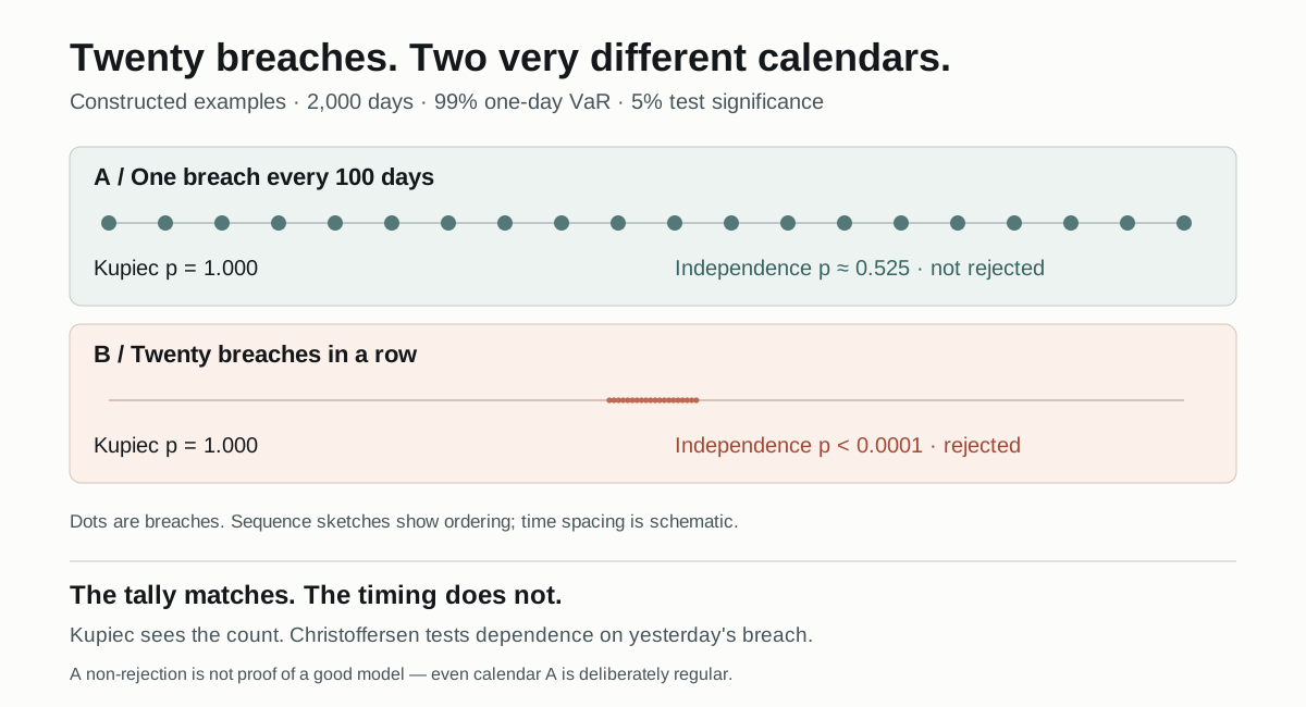
Imagine two risk reports landing on your desk. Each covers 2,000 trading days. Each uses a 99% one-day Value at Risk forecast. Each records exactly 20 occasions when the loss exceeded that forecast.

The exception count is almost offensively tidy: 1% of 2,000 is 20. Someone has already coloured both reports green.

Then you open the calendars. In the first report, the breaches are scattered across the sample. In the second, all twenty arrive on consecutive days. For four trading weeks, the forecast gets beaten every afternoon.

Should those reports get the same verdict? Kupiec's coverage test gives them the same result. Christoffersen's independence test does not. Let's build the two calendars, calculate the results, and see what that disagreement actually tells us. You can also run a VaR backtest in QuantLab as you read.

First, what counts as a breach?

A 99% one-day VaR of €2 million is a forecast of a loss threshold. Under the model, roughly 1% of days should have losses beyond that threshold. It is not a promise that €2 million is the most you can lose. The remaining 1% of the distribution has not politely agreed to stop there.

For each day, compare the forecast made before the outcome with that day's realised profit or loss. Record a 1 if the loss exceeds VaR, and a 0 otherwise. This is the exception sequence, also called a hit sequence.

With signed P&L, a profit is positive and a loss is negative. The comparison used here is:

boolean breach = -realisedPnl[t] > varForecast[t];

That minus sign matters. A €3 million profit should not trigger a loss exception because somebody compared absolute values.

Our example uses a strict “greater than” comparison and a constant forecast. For real data, align dates, currencies, horizons, and the P&L definition before calculating anything. A beautiful p-value computed against tomorrow's forecast is still an answer to the wrong question.

Two calendars, one count

We will construct the exception sequences directly. No market data, no claim that these are plausible eight-year trading histories. They are a controlled experiment: keep the count fixed and change only the timing.

Calendar A: one breach every 100 days, at positions 50, 150, …, 1950, using positions numbered from zero.

Calendar B: twenty consecutive breaches at positions 1000 through 1019. Every other day is a non-breach.

Both have 20 exceptions in 2,000 observations. Both start and finish with a non-breach, which also makes their transition counts easy to compare.

At a 99% confidence level, the forecast exception probability is 0.01. The observed fraction in both calendars is 20 / 2,000 = 0.01. So far, the two reports are indistinguishable.

Kupiec looks at the tally

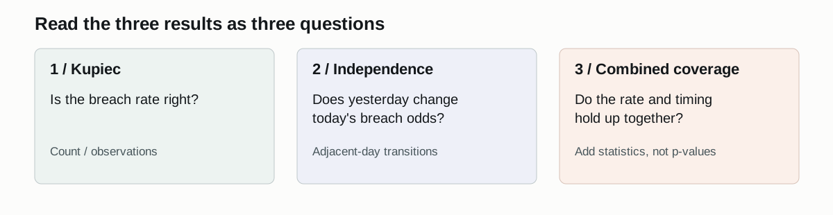
Kupiec's proportion-of-failures test compares the forecast exception rate with the observed rate. It asks whether allowing a different breach probability would explain the count substantially better.

Here, that freedom buys nothing. The observed rate is already exactly the forecast rate, so the likelihood-ratio statistic is zero and the p-value is 1.000 in both cases.

Move the breaches around however you like: keep 20 out of 2,000 and the Kupiec result stays the same. The test never sees the calendar.

This is useful, not a defect. If VaR is systematically too small, losses will tend to exceed it too often. A count test can detect that. It can also reject a forecast whose exceptions are too rare: an excessively conservative threshold is not necessarily a well-calibrated one.

But p = 1 does not mean a 100% probability that the model is correct. It means this particular statistic provides no evidence against the specified exception rate. That distinction is where the green highlighter needs a little supervision.

Christoffersen reads yesterday's entry

Christoffersen's first-order independence test asks whether today's breach probability changes depending on whether yesterday was a breach. It counts four kinds of adjacent-day transition:

Yesterday → today	Calendar A: spaced	Calendar B: clustered
No breach → no breach	1,959	1,978
No breach → breach	20	1
Breach → no breach	20	1
Breach → breach	0	19

Each column sums to 1,999 transitions. There are 2,000 observations, but the first one has no previous day inside the sample.

For Calendar B, the conditional probabilities are striking:

• After a non-breach: 1 / 1,979, about 0.051%.
• After a breach: 19 / 20, or 95%.

Yesterday is suddenly very informative. Once the streak starts, another breach is overwhelmingly likely in this constructed sample.

The test compares a model with one shared probability against a model with separate probabilities after breach and non-breach days. For the cluster, the separate probabilities explain the sequence much better.

Here are the results, calculated from the explicit transition counts using the likelihood-ratio formulas and their usual asymptotic chi-square references:

Result	Calendar A: spaced	Calendar B: clustered
Kupiec statistic	0.000	0.000
Kupiec p-value	1.000	1.000
Independence statistic	0.404	198.865
Independence p-value	0.525	about 3.69 × 10⁻⁴⁵
Conditional coverage p-value	0.817	about 6.56 × 10⁻⁴⁴

At a preselected 5% significance level, the clustered sequence rejects independence. The spaced sequence does not.

One possible explanation for clustering in real data is a volatility forecast that responds too slowly when conditions change. These counts alone cannot establish that cause. Data problems, changing exposures, and other model weaknesses deserve investigation too.

The spaced calendar has a secret

Calendar A is not random. It has an exception every hundred days, with the punctuality of a subscription renewal. A person looking at the complete sequence could spot that pattern.

Yet the first-order independence test does not reject it here. After a breach, the observed next-day breach rate is zero; after a non-breach, it is about 1%. With only twenty breach days, that difference is not large enough for this test to reject at 5%.

This is why “passes Christoffersen” is not a certificate of randomness. The test targets dependence on the previous day's breach state. It does not exhaust every possible pattern, longer lag, or source of predictability.

The example gives us both lessons at once: a count can miss an obvious cluster, and an independence test can miss a different kind of obvious pattern. Plot the sequence as well as reading the test output.

What conditional coverage adds

Conditional coverage combines the Kupiec and independence statistics:

conditional coverage statistic = coverage statistic + independence statistic

Its usual reference distribution has two degrees of freedom, whereas each individual test uses one. Add the statistics, not the p-values.

Because Kupiec is zero in our example, the combined statistic equals the independence statistic. Their p-values still differ because the reference distributions differ. The combined test rejects the cluster too.

In another sample, the breach rate could be wrong without obvious clustering, or both features could be wrong. Keeping the component results visible helps explain a rejection instead of reducing the investigation to one red tile.

Give the calculator a difficult afternoon

Open the QuantLab VaR backtesting calculator. Its normal controls generate a synthetic P&L series; they do not load your desk's historical data.

Start with confidence at 99%, a 2,000-day window, realised volatility multiplier at 1, and a zero-day stress window. Run it and note all three p-values. The random exception count need not equal twenty. Twenty is an expectation, not an appointment.

Next, introduce a 20-day stress window and increase the stress multiplier. Keep the seed fixed. This creates a period of extra volatility near the start of the simulated series. Inspect what changes. This experiment can change both the breach count and the clustering; it does not reproduce our equal-count calendars by itself.

For the exact example above, the calculator exposes editable Java source. Set the window to 2,000 and confidence to 99%, then replace the generated for loop that fills hit and increments x with:

for (int t = 0; t < n; t++) {
    hit[t] = t % 100 == 50;  // Calendar A
    if (hit[t]) x++;
}

Run it, then change just the assignment:

hit[t] = t >= 1000 && t < 1020;  // Calendar B

Leave the source's test functions in place. The result tiles round small p-values to 0.000; they are very small numbers, not mathematical zeros. Changing a form control regenerates the source, so finish the settings before making the edit.

What to check before trusting the verdict

A high p-value means “not rejected by this test,” not “validated.” At 99% confidence, a 250-day sample has only 2.5 expected breaches. There may be very little information about what happens after a breach. The chi-square references used here are asymptotic approximations; sparse transition counts make their finite-sample behaviour worth checking.

The breach sequence also discards loss magnitude. Losing just beyond VaR and losing ten times VaR both contribute one hit. Coverage tests alone cannot tell you how severe the losses beyond the threshold are.

For a practical review, keep the forecast and P&L series beside the exception plot. Check when the forecasts were produced, investigate the cluster dates, and report the component statistics alongside the chosen significance level. These academic tests are not a regulatory capital traffic-light calculation.

The two green reports can now go back to their owners with a better question: what happened on the days the forecast stopped keeping up? The count got us to twenty. The calendar told us where to look.

For the implementation walkthrough, continue with Backtesting a VaR model. For the experiment, return to QuantLab.

References

• Paul Kupiec, Techniques for Verifying the Accuracy of Risk Measurement Models, 1995: the proportion-of-failures coverage test.
• Peter Christoffersen, Evaluating Interval Forecasts, 1998: independence and conditional coverage tests.
• NablaTensor VarBacktest source: exception counting and test implementation.