13 billion Black-Scholes paths a second — with every Greek — on a laptop iGPU

Here is a number, and then the honest version of it.

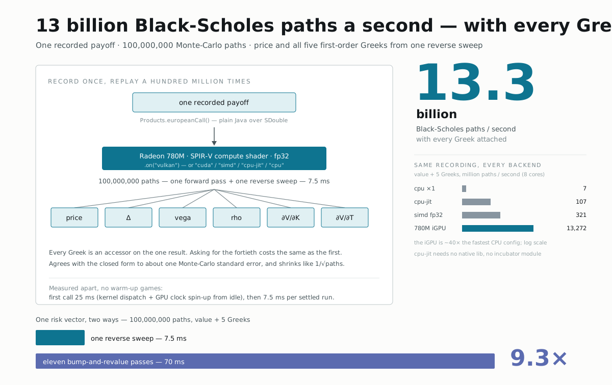
A European call, priced by Monte Carlo: one hundred million paths, and from each path the price and delta, vega, rho, strike sensitivity and time decay — all five first-order Greeks — read off a single reverse sweep. On the integrated GPU of a mid-range laptop (an AMD Radeon 780M, the graphics that ship on the same die as the CPU), that whole thing takes 7.5 milliseconds. Call it 13 billion Black-Scholes paths a second, with every Greek attached.

The "with every Greek" is the part that matters, and we'll get to why. First, what this is not: it is not the closed-form Black-Scholes formula. That formula exists, it's exact, and on a CPU core it runs at a few hundred million prices a second (more on that at the end). The reason to simulate a European — a contract that has a closed form — is that the exact same recording, with one line changed, prices an Asian, a barrier, an autocallable, a whole netting set: payoffs where no closed form exists and Monte Carlo is the only option. The European is the one you can check against arithmetic, which is the whole point of the demo.

The middle of it, in text, is where the numbers land:

                 adjoint MC     closed form        |diff|
   price            9.41191         9.41340      1.49e-03
   delta            0.59872         0.59871      9.15e-06
   vega            38.65737        38.66681      9.44e-03
   rho             50.45963        50.45723      2.40e-03
   dV/dK           -0.50460        -0.50457      2.34e-05
   100,000,000 paths, one run, on vulkan

   13.3 billion Black-Scholes paths/s  —  with every Greek  —  on AMD Radeon Graphics
   first call 25 ms (one-off), then 7.5 ms/run   ·   100,000,000 paths, value + 5 Greeks
   1 sweep 7.5 ms  vs  11 bump passes 70.3 ms  =  9.3x  (+2 passes per factor)

Six numbers on the left, six on the right, agreeing to four or five significant figures. The gap is Monte-Carlo sampling noise at a hundred million paths — about one standard error on the price, five figures on the Greeks — and the demo's convergence act (further down the recording) watches it shrink like 1/√paths.

The Greeks are the point, not a footnote

The last line of that block is the argument. In code the whole thing is one builder and one call:

EquityMarket market = EquityMarket.atmOneYear();          // S0 = K = 100, sigma 20%, r 3%, T 1y

try (MonteCarlo<EquityMarket> mc = MonteCarlo.of(Products.europeanCall())
        .market(market)
        .steps(1)                 // a European only needs the terminal value
        .greeks()                 // forward pass + one reverse sweep
        .on("vulkan")             // or .fastest(), "cuda", "cpu-jit", "simd"
        .build()) {               // records the tape, compiles the kernel — once

    Nabla.TypedValuation<EquityMarket> p = mc.run(100_000_000L, /*seed*/ 42L);

    double price = p.price();
    double delta = p.greek(EquityMarket::spot);   // dV/dS0
    double vega  = p.greek(EquityMarket::vol);    // dV/dsigma
    double rho   = p.greek(EquityMarket::rate);   // dV/dr
    // ...EquityMarket::strike, ::maturity — same one run.
}

The same recording compiles two ways: .greeks(), which does the forward pass and one reverse sweep, and .priceOnly(), which does the forward pass alone. Getting the five Greeks the usual way — shift each input a little, reprice, take a central difference — is 1 + 2×5 = 11 full Monte-Carlo passes. Here that's 70 ms against the adjoint sweep's 7.5 ms: a 9.3× gap, on a payoff with a closed form to keep everyone honest.

We've made the general version of this argument at length — across eight payoffs and three backends, the reverse sweep costs a small constant on top of the price while bump-and-revalue costs 1 + 2N and grows with every risk factor you add. What's new here is the scale: the reverse sweep isn't just cheaper per Greek, it's cheap enough that a hundred million paths' worth of a full first-order risk vector fits in under 8 ms on hardware that costs nothing extra. The headline isn't "fast pricing". It's "fast pricing and the whole risk vector, from the same run, for about the cost of the price alone."

No warm-up games

Every "N per second" GPU benchmark you've read quietly warmed up first. This one says so out loud, because on an integrated GPU the warm-up is a large part of the story: the chip drops to a low clock when idle, and the first launch after a pause can be 40× slower than the settled rate — a few hundred milliseconds, not seven.

Hiding that behind a warm-up burst and quoting the best of twenty runs would have produced a bigger, less honest number. Instead the demo runs the sweep two dozen times and reports two things separately:

• first call: 25 ms — the one-off. Kernel dispatch, and the GPU clock spinning up. If you run the demo cold, straight after boot, you'll see this read higher; it's a live measurement, not a constant.
• then 7.5 ms/run — the settled per-run time, the median of the runs once the clock is up. This is what a real batch job — a risk run, a scenario grid, a book of millions of options — experiences, because a real batch job keeps the GPU busy the whole time.

The 13-billion headline is derived from the settled figure, and the adjoint-vs-bump ratio uses the settled figure on both sides. The first-call cost is disclosed, not amortised away.

The same recording, four backends

The payoff is recorded once. Where it runs is one method call. Same machine (a Ryzen 7 8845HS, 8 cores, AVX-512, and the 780M on the same die), same 100 M-path European, warmed and measured over many runs, in millions of paths per second:

backend / config	price-only	value + 5 Greeks
cpu — the scalar oracle, 1 thread	12	7
cpu — 8 threads	84	49
cpu-jit — generated bytecode, 8 threads	171	107
simd — JDK Vector API, fp64, 8 threads	463	167
simd — fp32, 8 threads	534	321
vulkan — the 780M iGPU, fp32	15,525	13,272

The iGPU is roughly 30–40× the fastest CPU configuration — not because the CPU path is slow (the best one does half a billion paths a second on eight cores) but because a Monte-Carlo path is exactly the dense, independent, transcendental-heavy arithmetic a GPU is built for. On the CPU side, fp32 on the Vector API is the fastest (16 lanes instead of 8), and cpu-jit at 171 / 107 is the one that needs no incubator module and no native library.

One row deserves a note. cpu is the scalar interpreter — it walks the recorded tape node by node instead of compiling it — and at 8 threads it does 84 / 49. cpu-jit runs the same tape as generated bytecode and does 171 / 107, about twice as fast. That gap is the cost of interpreting versus compiling; it is also the reason the interpreter exists only as the bit-exact reference the other three are checked against.

The tape isn't a tax

It's fair to ask what all that recording-and-compiling machinery costs versus just writing the Monte-Carlo loop by hand. We checked: a plain Java for-loop over double, using the same random-number generator and the same geometric-Brownian-motion step, no tape, no code generation.

approach	price, 1 thread	price, 8 threads	value + 5 Greeks, 8 threads
hand-written Java loop	25	191	—
hand-written, 5 pathwise Greeks hand-coded	24	182	182
cpu-jit — recorded, compiled from the tape	24	171	107

The generated kernel lands within about 10% of the hand-written loop. Recording the payoff and compiling a kernel from it is a one-off — around 11 ms for this payoff — not a per-run cost. What you get for it is: the same recording runs on cpu-jit, simd or the GPU with a one-line change, and every Greek falls out of one reverse sweep for any payoff you record, with no derivative code to write or get wrong. (Hand-coding the five pathwise derivatives is faster still — 182 versus 107 — but you write and maintain those five lines for every new payoff, and a barrier or a digital will punish a mistake in them. The tape's adjoint is exact for anything you can express.)

For scale: the closed form

Because someone will ask how this compares to a straight closed-form pricer: the analytic Black-Scholes formula, compiled with -O3 -march=native -ffast-math so the exponentials vectorise, runs at about 350 million prices a second on one core of this same machine, and around 2 billion a second across all sixteen threads. That's price-only, no Greeks, no random numbers, no path — a single cheap evaluation per option.

The GPU's 13 billion paths a second is doing something else entirely: a counter-based random draw, a Box-Muller transform, the model step and the payoff — roughly a hundred times the arithmetic per element — and carrying a five-way reverse sweep on top. Different jobs. Neither is a bottleneck for anything. The reason the Monte-Carlo path exists at all is the payoffs the closed form can't touch, and the reason it's worth putting on a GPU is that those payoffs, on a real book, come with a risk vector that used to mean an overnight batch.

Try it yourself

git clone https://github.com/nablatensor-dev/nablatensor && cd nablatensor
mvn -o -q compile
./demo/black-scholes-both-ways.sh --fast          # the narrated version, above

The demo picks the fastest backend it can actually run — CUDA, else Vulkan, else the generated CPU kernel — and prints which. On a laptop with no GPU it falls back to cpu-jit and the headline reads in the low hundreds of millions instead of billions; the reconciliation, the error ladder and the adjoint-vs-bump ratio are identical.

The non-narrated version is com.nablatensor.examples.BlackScholesBothWays. Run it with exec:exec — exec:java runs the class inside Maven's own JVM and holds all of its output until the end:

mvn -o -q -pl nablatensor-examples exec:exec -Dexec.executable=java \
  -Dexec.args="-cp %classpath com.nablatensor.examples.BlackScholesBothWays"

It reads -Dscenarios=, -Dengine=vulkan|cuda|cpu-jit|simd|cpu and -Dseed= — append them after the class name in exec.args.