MNIST in Java: train a digit recognizer, then inspect its mistakes

A handwritten 4 can look quite convincing as a 9. A single accuracy number hides that argument; a gallery of wrong predictions puts it back in view. This notebook trains a small neural network in Java, then shows the digits it misreads. The weights start random. There is no pretrained model behind the button.

Run the cells from the top, or choose Run all. Java executes in an emulated OpenJDK 27 JVM inside your browser; no account or JDK installation is needed. The notebook selects WebGPU when available, otherwise CPU, using jax4j 0.2.1 and its automatic differentiation. The model uses all 784 pixels from each 28×28 image. Full-resolution training can take several minutes; the live epoch messages show progress while the training cell runs.

Chrome/Edge flags: #force-enable-webgpu-interop / #enable-unsafe-webgpu. Firefox about:config: dom.webgpu.enabled=true. Relaunch afterwards.

Real digits, small enough to inspect

CVDF hosts the original compressed MNIST files with permission from Yann LeCun. The four gzip files total about 11.1 MiB. MNIST has 60,000 training images and 10,000 test images, each 28×28 grayscale pixels. Downloading the data and training on it are different costs: images compress well; matrix multiplication still has work to do.

Our reproducible subset manifest records the source checksums, seed and original sample indices. We package 10,000 training images, 1,000 validation images taken from the remaining official training data, and 1,000 test images from the official test set. Each packaged split has equal counts of the ten labels. The training portion compresses to about 1.65 MB.

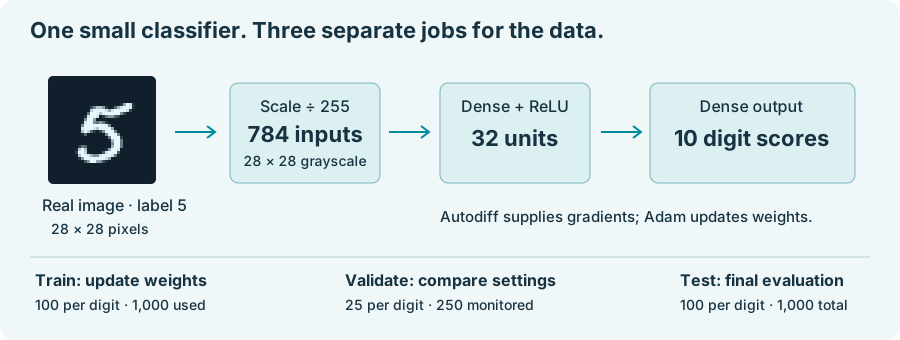
The browser default selects 1,000 training images: 100 per digit. Monitoring uses 250 validation images: 25 per digit. The test set has 100 per digit, and the sample gallery shows one image per digit. Validation helps choose settings; test images are reserved for the final cell. The loader and batching helper are available as Java source. They contain no handwritten backpropagation or synthetic replacement digits.

selectTarget("webgpu") prefers the browser GPU and selects CPU if initialization fails. Use "cpu" to force CPU. This convenience method belongs to the notebook adapter; select the target before creating tensors.

The pictures above come from the loaded training data. The custom notebook resource brings compressed data and a small helper into the guest JVM.

Keep every pixel

We divide pixel intensities by 255, then flatten the 28×28 image into 784 features. Every original pixel reaches the network: pool = 1 means no averaging or downsampling. These inputs feed 32 hidden units and ten output scores. The gallery displays the same full-resolution images the model receives.

The training budget stays small: 1,000 images and eight epochs. Choose training counts in multiples of ten so every digit has the same number of images. Full-resolution inputs require more computation than a reduced image. Restart the kernel before changing the configuration so the model and optimizer start together again. The dataset and runtime remain in browser memory only; reloading discards edits and Java state.

parameters contains two weight matrices and two bias vectors. The seed makes initialization repeatable. Each batch has shape [batch,784], while its labels have shape [batch,10]: a one-hot label has a one at the correct digit and zeros elsewhere. The helper shuffles the selected training rows every epoch, using a reproducible seed, and closes each temporary batch afterwards.

Write the network, let autodiff do the backward pass

A dense layer multiplies its input by weights and adds a bias. ReLU replaces negative activations with zero; that nonlinearity lets the second layer express more than another linear map. The output scores are logits, not probabilities.

Softmax turns logits into a probability distribution. Cross-entropy penalizes a model that assigns low probability to the correct label. We compute log-probabilities directly, subtracting each row's maximum before exponentiation. This avoids exponential overflow without adding an arbitrary epsilon to the loss.

Var records differentiable operations. The training cell asks jax4j for the four parameter gradients; it never writes the derivatives of matmul or ReLU. For monitoring, scoreLoss uses a separate double-precision cross-entropy reduction over the model's F32 logits. It reads the same fixed 250 class-balanced validation images after each epoch. That makes the monitoring curve comparable over time.

Keep the optimizer's memory

Adam maintains moving averages of gradients and squared gradients. Recreating that state on every batch would change the algorithm. Here, optimizerState travels from one update to the next, alongside the model parameters. The old tensors are closed only after the replacement state has been produced. The browser GPU bridge cannot compile generated JIT kernels, so its update uses the helper's eager Adam operations with the same moments and bias correction. CPU uses FunctionalAdam's compiled update. GPU execution errors stop the cell.

Uniform probabilities would give a loss of ln(10) ≈ 2.3026. Random weights need not produce uniform probabilities or exactly that value. Epoch zero below is a real measurement of the initialized model.

The next cell performs 32 updates with the defaults: four batches per epoch, eight epochs; the final batch has 232 images. Each epoch prints its loss as soon as it completes. Use Stop to terminate a long run; that destroys the kernel, so restart from cell one afterwards. Emulated CPU timings are not native Java benchmarks.

The training curve averages minibatch losses as the model changes during an epoch. The validation curve evaluates the final model of that epoch on fixed images. Those are different measurements; their relative heights alone do not diagnose a bug. If training loss falls while validation loss rises consistently, the model may be fitting training details that do not generalize.

Read the wrong answers

Now load the held-out test subset. Rows of the confusion matrix are actual labels; columns are predictions. Diagonal counts are correct. The gallery shows the one example per digit: the first error in test order for that digit, or the first correct example if that digit has no errors. Accuracy describes these 1,000 images, not the full official test set or handwriting collected from a different population.

Data credit: Yann LeCun, Corinna Cortes and Christopher J. C. Burges. Sources: MNIST distribution and gzip downloads, dataset structure and original split, and gradient-based document recognition. The data provenance notice distinguishes the images from the Apache-2.0 helper code.