ISDA SIMM Portfolio Margin: A Worked Example

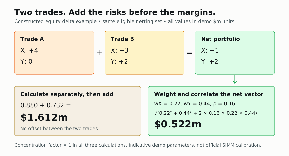
Two trades arrive with their own margin estimates. The first needs $880,000. The second needs about $732,000. Add them to the same eligible portfolio and the combined estimate is about $522,000.

The spreadsheet that adds the two trade margins asks for $1.612 million. The portfolio calculation asks for less than either trade alone. Both calculations used the same inputs. Where did the other million go?

It went away before the final margin number existed: one trade offset part of the other's sensitivity. The remaining exposures then went through a correlation calculation. Those are two separate mechanisms, and mixing them up makes a hedge look more mysterious than it needs to be.

We will construct the inputs directly and reproduce the numbers in the QuantLab SIMM calculator. These are teaching numbers, not quotes for real trades or an approved collateral calculation.

Two trades, two risk factors

A sensitivity measures how a position's value responds to a market move. Delta is the first-order response; equity delta concerns changes in an equity price. SIMM, the ISDA Standard Initial Margin Model, uses market-risk sensitivities as inputs to its margin calculation. ISDA describes that sensitivity-based approach in its margin optimisation presentation.

For this experiment, imagine two equity positions, A and B, in the same eligible netting set: the group of transactions whose risks may be combined for this calculation. Both have exposure to the same named equity factor X; B also has exposure to factor Y. X and Y sit in equity bucket 1. A bucket groups factors for aggregation.

Delta sensitivity, demo $m units	Factor X	Factor Y
Trade A	+4	0
Trade B	−3	+2
A + B	+1	+2

These vectors are constructed inputs, not sensitivities obtained by pricing specified contracts. We assume all other sensitivities are zero, including vega (volatility sensitivity) and curvature (the nonlinear response left after accounting for delta). That keeps every dollar in the example traceable to this table.

The calculator uses an indicative, scoped parameter set inspired by the engine's demoV26() tables. It is not the official SIMM v2.6 calibration, nor a claim to implement the current published version. For equity bucket 1, its Java source sets the delta risk weight to 0.22, within-bucket correlation to 0.16, and delta concentration threshold to 8, in the demo's million-dollar units. We will use those exact settings.

Net first, weight second

Add sensitivities that refer to the same risk factor before calculating margin. Factor X becomes 4 − 3 = 1. Factor Y remains 2. A trade identifier is not a market-risk factor: calling the entries A#X and B#X would prevent this implementation from recognising that both positions respond to X.

Below the concentration threshold, the risk weight turns the combined sensitivities into weighted sensitivities:

wX = 0.22 × 1 = 0.22
wY = 0.22 × 2 = 0.44

For these two distinct factors in one bucket, the demo delta aggregation is:

K = sqrt(wX² + wY² + 2 × rho × wX × wY)

The cross term appears twice in the implementation's double loop, hence the 2. Here rho = 0.16. There is only one bucket and one risk class with nonzero exposure, so its delta margin is also the entire portfolio margin in this deliberately narrow experiment.

Calculate the trades separately, then together

Trade A has only factor X. Its margin is simply 0.22 × 4 = 0.880.

Trade B has weighted sensitivities −0.66 and +0.44. Their opposite signs make the correlation term negative:

K_B = sqrt(0.66² + 0.44² + 2 × 0.16 × (−0.66) × 0.44)
    = 0.732306

For the combined portfolio, both residual weighted sensitivities are positive:

K_AB = sqrt(0.22² + 0.44² + 2 × 0.16 × 0.22 × 0.44)
     = 0.522471

Calculation	Demo margin ($m)
A alone	0.880000
B alone	0.732306
Sum of standalone margins	1.612306
A and B aggregated together	0.522471

The combined margin is about 67.6% below the standalone sum. This is not an observed saving from a trading desk. It is the result of the fixed vectors and demo parameters above.

Notice what happened to the correlation term: it became positive in the combined portfolio, even though margin fell. The large reduction came from removing three units of X exposure by netting. Correlation then aggregated what survived. A single “diversification benefit” number hides that sequence of events.

A negative incremental margin is possible

If A is already in the portfolio, what does adding B cost? Subtract the original portfolio margin from the new one:

incremental margin of B = 0.522471 − 0.880000 = −0.357529 $m

In this example, B releases about $358,000 of model margin even though its standalone margin is positive. Its offset to X more than compensates for the additional Y exposure.

That does not turn B into a risk-free trade. It has price risk, and the portfolio still has residual exposure. Nor is incremental margin an intrinsic property of B: put it into a different starting portfolio and the answer changes.

Order matters for assigning incremental contributions. Starting with B instead, adding A changes margin by 0.522471 − 0.732306 = −0.209835. Each path reaches the same final total, but allocates the journey differently. If a desk wants trade-level allocations that sum to portfolio margin, it needs an allocation convention; standalone margins will not do that job automatically.

An opposite sign is not always an exact hedge

Replace B with a position containing only −3 units of X. The combined sensitivity is +1 unit of X, and margin is 0.220. Replace it with −4 units of X and the delta-only example nets to zero.

Now move that −3 sensitivity to a different factor Y in the same bucket. There is no exact factor netting. The combined vector is (4, −3):

K = 0.22 × sqrt(4² + (−3)² + 2 × 0.16 × 4 × (−3))
  = 1.012000 $m

It is below the standalone sum of 0.880 + 0.660 = 1.540, but well above 0.220. Correlation provides a partial offset between distinct factors; it does not erase them as though they were identical.

Even the zero result for an exact X hedge applies only to our delta-only inputs. Two real options can offset delta while leaving vega or curvature. Compare the full sensitivity vectors before celebrating the empty margin tile.

Reproduce it in the Java editor

Open Compute ISDA SIMM Initial Margin. The normal form lets you add or remove trades and edit their IDs, counterparties, product classes, notionals and sides, plus simulation scenarios and seed. It does not offer a direct sensitivity-grid input.

The generated example combines synthetic factors with actual option repricing for the first equity trade, or the first trade if no equity trade exists. Its synthetic factors depend on row order and include trade IDs in factor names. Deleting rows and comparing the default results therefore would not hold our two vectors fixed.

For the controlled experiment, finish any form changes, then replace only the generated main method in the Java editor with this one. Leave the parameter arrays and helper methods, including margin, intact:

public static void main(String[] z) {
    RiskFactor x = RiskFactor.equityDelta("1", "X");
    RiskFactor y = RiskFactor.equityDelta("1", "Y");
    Sensitivities a = Sensitivities.builder()
        .add(x, 4.0).build();
    Sensitivities b = Sensitivities.builder()
        .add(x, -3.0).add(y, 2.0).build();
    Sensitivities portfolio = a.plus(b);
    double ka = margin(a, 3, RiskMeasureEnum.DELTA);
    double kb = margin(b, 3, RiskMeasureEnum.DELTA);
    double kab = margin(portfolio, 3, RiskMeasureEnum.DELTA);
    System.out.println("A alone $m: " + ka);
    System.out.println("B alone $m: " + kb);
    System.out.println("Standalone sum $m: " + (ka + kb));
    System.out.println("Incremental B $m: " + (kab - ka));
    for (int c = 0; c < RC.length; c++) {
        double delta = c == 3 ? kab : 0.0;
        System.out.println("CLASS|" + RC[c] + "|" + delta + "|0|0");
    }
    String[] products = {"RATES_FX", "CREDIT", "EQUITY", "COMMODITY"};
    for (String p : products) {
        double delta = p.equals("EQUITY") ? kab : 0.0;
        System.out.println("PRODUCT|" + p + "|" + delta + "|0|0|" + delta);
    }
    System.out.println("TOTAL|" + kab);
}

Click Compute SIMM. The log reports the standalone comparisons; the result tables and total tile report the combined portfolio. The tile rounds to 0.522 $m. This edited calculation does no simulation, so scenarios and seed do not affect it. Changing a form control regenerates the source and discards the manual edit.

When scale changes the rules

The demo's concentration factor is:

CR = max(1, sqrt(abs(sum of bucket sensitivities) / threshold))

Our bucket sums are 4 for A, −1 for B, and 3 together. All have absolute values below 8, so CR = 1 throughout. Concentration contributes none of the reduction we calculated.

Try a single factor X with sensitivity 8, then 16. At 8, margin is 0.22 × 8 = 1.760. At 16, the concentration factor becomes sqrt(16 / 8) = sqrt(2), so margin is about 4.978. Doubling sensitivity has multiplied margin by about 2.828.

These results describe the calculator's simplified bucket-sum rule. Official SIMM concentration rules depend on risk class and factor structure; this demonstration is not a substitute for those specifications. It does show why a margin estimate at one size cannot always be scaled linearly to another.

Keep the portfolio boundary visible

The calculator's counterparty column is descriptive: the generated Java counts counterparties but aggregates every row into one sensitivity vector. Changing that label does not create separate netting sets. Our combined result assumes A and B are eligible to be aggregated together.

For positions that must be calculated separately, the relevant comparison here is the standalone sum, $1.612m. A dashboard total is not permission to combine exposures across unrelated counterparties. ISDA's collateral operational practices also identify disagreements in product-class, risk-class and bucket mapping as possible sources of margin disputes.

For an actual portfolio review, keep the eligible grouping, market snapshot, sensitivity units and parameter version alongside the result. Then compare the vectors before and after the proposed trade. That makes a negative incremental margin explainable: in our example, three units of X disappeared, and two units of Y remained.

Continue with the SIMM implementation lesson for the wider demonstration book, or return to QuantLab to change the vectors yourself.

References

ISDA SIMM methodology publications: official versioned specifications; the calculator uses indicative demo parameters.
NablaTensor Sensitivities: factor-wise addition used by a.plus(b).
NablaTensor NestedAggregation: weighted, correlated bucket aggregation used for the numerical example.

ISDA SIMM: Why Portfolio Margin Isn’t the Sum of Trade Margins