BA-CVA Worked Example: From Exposures to Capital

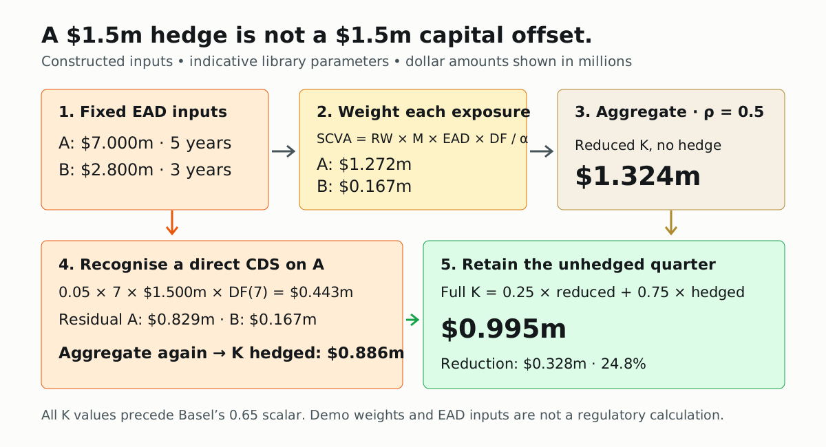
Buy $1.5 million of credit protection on a counterparty. The BA-CVA calculation falls by about $328,490. The protection's notional is larger than the original $1.324 million charge, yet the charge is nowhere near zero.

Where did the rest of the hedge go? Through a maturity adjustment, a risk weight, a portfolio aggregation and a blend with the unhedged result. The notional never entered the calculation as a dollar-for-dollar capital offset. That would have made this a rather short article.

We will build a two-counterparty example with fixed exposure inputs and reproduce it in the QuantLab BA-CVA calculator. These are constructed teaching numbers, using the library's indicative parameters. No simulated portfolio results are being presented as observations.

Decide which number you are calculating

CVA, or credit valuation adjustment, measures the reduction in a portfolio's value associated with possible counterparty default. A CVA risk capital calculation addresses the risk that the adjustment changes. The CVA amount and its capital charge are different outputs.

BA-CVA is the basic approach to that capital calculation. It combines exposure at default, maturity and counterparty risk weights. The BA-CVA lesson covers the wider approach; here the question is narrower: how does each exposure input survive the journey to the final number?

Our reference is the Basel Committee's MAR50 framework published on 8 July 2020, effective 1 January 2023. Its reduced and full capital requirements apply a 0.65 scalar to K_reduced and K_full. The calculator reports the library's K values before that scalar. We use that convention throughout the worked example.

The library's rating-by-rating risk weights are also indicative. Its BBB financial weight is 5.75%; the cited Basel table assigns 5% to investment-grade financials. Matching the demo's output therefore does not reproduce an official regulatory submission. Applying 0.65 alone would not fix the parameter difference.

Start with two exposure rows

A netting set groups transactions for which exposure can be calculated together under the relevant netting arrangement. Assume one netting set per counterparty, with every amount expressed in dollars:

Input	CPTY-A	CPTY-B
Library rating and sector	BBB financial	A corporate
Effective maturity, years	5	3
Exposure at default, EAD	$7,000,000	$2,800,000
Indicative risk weight, RW	0.0575	0.0300

EAD is the exposure measure supplied to the capital formula, not the sum of trade notionals. Our values are fixed assumptions. We have not derived them from specified swaps or claimed that either is an approved exposure calculation.

QuantLab normally supplies a demonstration proxy: EAD = alpha × expected positive exposure, with alpha = 1.4. Under that convention our EADs correspond to expected positive exposures of $5 million and $2 million. Those are convenient explanatory equivalents, not simulated results. Actual regulatory EAD follows the applicable counterparty-credit-risk methodology; the proxy is not a substitute for that process.

Keeping EAD fixed makes the next steps auditable. A new seed cannot move our starting point while we are trying to understand a risk weight.

Turn exposure into a counterparty contribution

The library calculates each row's stand-alone contribution, SCVA, as:

DF(M) = (1 − exp(−0.05 × M)) / (0.05 × M)
SCVA = RW × M × EAD × DF(M) / alpha

DF is the supervisory maturity discount. The 0.05 is fixed in this implementation; it is not the calculator's short-rate setting. For our maturities, DF(5) = 0.884797 and DF(3) = 0.928613. The cited Basel rules distinguish this non-IMM discount treatment from the Internal Models Method, where DF = 1.

For A:

SCVA_A = 0.0575 × 5 × 7,000,000 × 0.884796868 / 1.4
       = $1,271,895.50

For B:

SCVA_B = 0.03 × 3 × 2,800,000 × 0.928613490 / 1.4
       = $167,150.43

These are weighted capital inputs, not CVA valuations. If you started from the demo proxy EAD = 1.4 × EPE, the division by alpha would cancel that multiplier. Do not multiply by 1.4 again after supplying EAD.

The implementation adds row contributions sharing the same counterparty ID before portfolio aggregation. With several netting sets for A, calculate their maturity-adjusted contributions separately, then sum them into SCVA_A. Averaging their maturities first generally changes the answer: M × DF(M) is nonlinear.

Aggregate the counterparties

Adding our two contributions gives $1,439,045.93. The reduced calculation instead uses rho = 0.5:

K_reduced = sqrt((rho × (SCVA_A + SCVA_B))²
                 + (1 − rho²) × (SCVA_A² + SCVA_B²))
          = $1,323,614.88

The shared component is the square of the weighted sum. The second component combines the individual squares. Together they recognise imperfect co-movement across counterparties.

There is an easy two-name cross-check:

K_reduced² = SCVA_A² + SCVA_B² + 2 × rho² × SCVA_A × SCVA_B

The cross term uses rho² = 0.25, not rho = 0.5. Substituting 0.5 there would produce a different number while still looking reassuringly like a correlation formula.

A also dominates this portfolio. B's much smaller contribution cannot provide the same diversification effect as a second contribution of comparable size. Counterparty count alone says little about the reduction.

Give the CDS its own calculation

Now assume an eligible single-name credit default swap, or CDS, directly referencing CPTY-A. Use the calculator's existing hedge settings: $1.5 million notional, seven-year remaining maturity, 0.05 hedge risk weight and reference correlation 1.0.

The MAR50 hedge rules require eligible instruments to mitigate counterparty credit-spread CVA risk and be managed for that purpose. The demo accepts an assumed hedge; it does not establish eligibility or model the protection seller's exposure.

Its discounted weighted magnitude is:

H = RW_hedge × M_hedge × notional × DF(M_hedge)
  = 0.05 × 7 × 1,500,000 × 0.843748315
  = $442,967.87

There is no division by alpha in this hedge expression. With a direct reference, the full magnitude offsets A's contribution. The library's hedge-misalignment term is zero because the reference correlation is one. We have no index hedge.

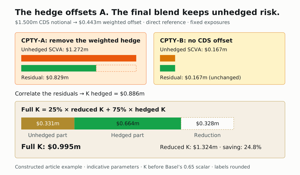
A's residual becomes $1,271,895.50 − $442,967.87 = $828,927.63. B stays at $167,150.43. Put those residuals through the same aggregation:

K_hedged = $885,628.64
K_full   = beta × K_reduced + (1 − beta) × K_hedged
         = 0.25 × 1,323,614.88 + 0.75 × 885,628.64
         = $995,125.20

Output, before the Basel scalar	Value
Reduced K, without hedge recognition	$1,323,614.88
Hedged component	$885,628.64
Full K, including the unhedged blend	$995,125.20
Reduced K minus full K	$328,489.68

The full result falls by about 24.8%. The reduced result stays fixed: that calculation does not recognise the CDS. Even if the hedged component reached zero, beta = 0.25 would leave one quarter of reduced K. Hedging A alone also leaves B's exposure.

Reproduce the numbers in QuantLab

Open Compute the BA-CVA Fallback Charge. The form controls two counterparty credit inputs, recovery, short rate, CDS notional, exposure paths and seed. Ratings, sectors, swap books and hedge maturity are set in the generated Java source; there is no EAD grid in the form.

Set CDS notional to 1500000. Finish all form changes, then find the line declaring BaCva.Exposure ea and eb in the Java editor. Replace those two declarations with:

BaCva.Exposure ea = new BaCva.Exposure(a, 5.0, 7_000_000.0);
BaCva.Exposure eb = new BaCva.Exposure(b, 3.0, 2_800_000.0);

Leave the surrounding code intact and click Compute BA-CVA capital. The counterparty table should round SCVA to 1,271,895 and 167,150; the reduced and full tiles should show 1,323,615 and 995,125.

This edit freezes only the BA-CVA inputs. The program still runs its exposure simulations, and its CVA and SA-CVA outputs still describe the original simulated swap books. They are not comparisons for our constructed exposure table. Paths and seed can change those outputs; they cannot change our fixed BA-CVA calculation.

For an unhedged check, change the hedge builder's notional in the editor to .notional(0.0). Full K should equal reduced K. Changing a form control regenerates the source, so reapply the exposure declarations if you use the form to change the hedge instead.

Two useful changes to the experiment

First, change A's rating in the Java builder from BBB to BB while retaining the fixed exposure declarations. The library's risk weight rises from 0.0575 to 0.12. Reduced K becomes $2,701,031.29, with no new EAD calculation required. This jump belongs to the indicative lookup; it is not evidence that the exposure itself doubled.

Second, hold the original ratings and increase the CDS notional. The library squares residual contributions, so a sufficiently large hedge can drive A's residual negative and eventually increase the hedged charge. A larger hedge is not automatically a smaller capital number. The hedging CVA lesson explores reference mismatch and hedge sizing in more detail.

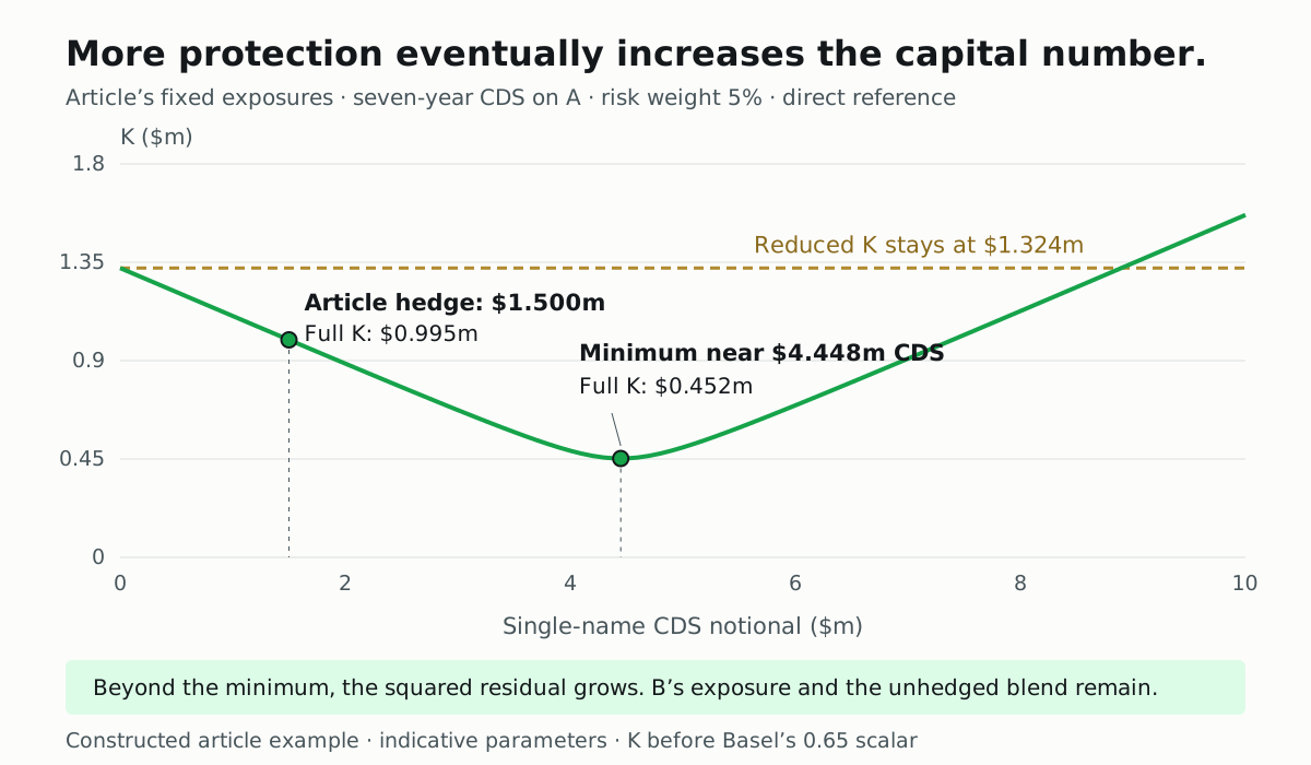
The curve holds our exposure table fixed. After applying the Java edits above, explore the same relationship in the QuantLab hedge-size graph. Its precomputed default results use the calculator’s simulated exposures, so their curve differs from this one.

For orientation, multiplying our original K results by 0.65 gives $860,349.67 and $646,831.38. These remain illustrative scaled values: the risk weights and constructed exposure assumptions have not become regulatory inputs by acquiring another decimal place.

A useful calculation record keeps the EAD method, netting-set boundaries, effective maturities, parameter version, hedge eligibility and scalar convention next to the result. Here that record explains the entire $328,490 reduction: a $442,968 weighted hedge offset A, the residuals were aggregated, and the full formula retained its unhedged quarter.

References

• Basel MAR50, published July 2020 and effective January 2023: paragraphs 50.14–50.26 specify reduced/full BA-CVA, weights, discounting and hedge recognition.
• NablaTensor BaCva: counterparty grouping and aggregation used here.
• NablaTensor BaCvaParameters and CvaHedge: indicative weights and discounted hedge magnitude.